

Loading…
Loading…
Loading…
Eduqas GCSE Geography A · C111
Eduqas C111 · Statistical Skills Check the specification (PDF) (opens in a new tab)
A fieldwork investigation may produce many measurements, such as sediment sizes or river depths. Statistical summaries help you compare places without listing every observation. Central tendency describes a typical value, while spread describes how much the observations vary. Two sites can have the same average but very different spreads, so a useful comparison often needs both.
The mean shares the total equally between all observations:
For a frequency table, multiply each value by its frequency before adding the results. Consider this household car-ownership table:
| Cars per household | Frequency |
|---|---|
| 1 | 2 |
| 2 | 15 |
| 3 | 6 |
There are households and cars. The mean is cars per household. An average need not be a value that any individual household actually has.
The median is the middle value after the observations have been put in order. With an odd number of observations, select the middle one; with an even number, average the two middle values. In the car table, observations 1–2 have one car, observations 3–17 have two, and observations 18–23 have three. The middle observation is the 12th, so the median is two cars.
The mode is the most frequent value: here it is also two cars. A dataset can have more than one mode if values tie for the greatest frequency. For grouped observations, you usually identify a modal class rather than an exact mode. For example, if the age classes 0–under 10, 10–under 20, 20–under 30 and 30–under 40 have frequencies 12, 15, 2 and 11, the modal class is 10–under 20 years.
The mean uses every value, making it useful for numerical comparisons, but an unusually large or small observation can pull it away from the main group. The median is often more representative when a few extreme values occur. The mode is useful when the question concerns the most common value or category.
The range measures the full distance between the smallest and largest values:
The range of car ownership in the table is cars. For grouped measurements, the exact extremes are unknown, so subtracting the lowest occupied class's lower boundary from the highest occupied class's upper boundary gives an estimate.
Quartiles divide ordered observations into quarters. The lower quartile, , marks approximately one-quarter of the way through the data; the upper quartile, , marks three-quarters. For a small ordered dataset, find the , then find the middle of each half, leaving out the overall median when there is an odd number of observations.
Consider these 15 ordered values:
.
The median is the 8th value, 12. The middle of the lower seven values is 5, and the middle of the upper seven is 14. Therefore and .
The interquartile range is:
Here it is , compared with a full range of . The IQR describes the middle 50% of observations, so extreme values affect it less than they affect the range. A smaller IQR indicates that the central observations are more closely clustered.
Cumulative frequency adds each frequency to all the frequencies before it. It tells you how many observations lie below successive class boundaries.
For example, these grouped worm-length measurements total 48 observations:
| Length, (mm) | Frequency | Cumulative frequency |
|---|---|---|
| 6 | 6 | |
| 14 | 20 |
Twenty worms are at most 30 mm long, while 46 are at most 40 mm long. This makes it possible to locate the class containing a median, quartile or other .
You can also plot cumulative frequency against each upper class boundary, starting at the lowest boundary with a cumulative frequency of zero. For this table, plot , , , and , with length in millimetres on the horizontal axis and cumulative frequency on the vertical axis. Join the points with an increasing curve.
To estimate a quartile from the graph, locate one-quarter or three-quarters of the total on the vertical axis, move across to the cumulative-frequency curve and then down to the measurement axis. Here those cumulative counts are 12 and 36. For the median, use half the total: 24. These readings estimate lengths, not frequencies.
Percentage change expresses a change relative to the starting value, allowing comparisons between populations of different sizes:
For example, a census table records 144,000 United States-born residents in 2001 and 177,000 in 2011. The increase is 33,000, so the percentage increase is .
A fall produces a negative result. The Republic of Ireland-born figures fell from 473,000 to 407,000: , or a 14.0% decrease.
When using a line graph instead of a table, first read the values at the two required dates, checking the vertical-axis units and scale. Then use the same calculation. If graph readings are approximate, the calculated percentage is approximate too.
A histogram shows how continuous measurements are distributed among class intervals. The horizontal axis shows the measured variable and its units. Each bar spans its actual class boundaries, and adjoining classes have no gaps between their bars.
With equal class widths, frequency can be used for the vertical axis. With unequal widths, use frequency density:
For the worm-length table, the class widths are 5, 10, 10 and 20 mm. Dividing each frequency by its width gives bar heights of 1.2, 1.4, 2.6 and 0.1 worms per millimetre. Choose a regular numerical scale on each axis, label both axes and draw each bar across its full class interval.
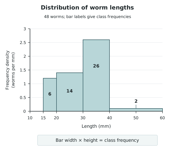
Unequal class widths require frequency density: each bar's area represents its class frequency.
Bar area, rather than height alone, represents frequency. The final class is twice as wide as the 30–40 mm class, but its much smaller height gives it an area representing only two worms. Where the axis shows frequency density, recover a frequency by multiplying bar width by height.
A normal distribution has a symmetrical bell shape: frequencies are greatest near the centre and decrease towards both ends. A histogram of approximately normal data follows this general pattern, although its bars need not be perfectly symmetrical.
For example, suppose sediment-length classes of 0–under 10, 10–under 20, 20–under 30, 30–under 40 and 40–under 50 mm have frequencies 2, 8, 14, 8 and 2. Mark the class boundaries at 0, 10, 20, 30, 40 and 50 mm, then draw adjoining equal-width bars with those frequency heights. The central peak and matching decrease on either side demonstrate an approximately normal shape. Do not join the bar tops into a line.
A skewed distribution is asymmetrical. A positively skewed distribution has a longer tail towards high values on the right; a negatively skewed distribution has a longer tail towards low values on the left. The tail, not the position of the tallest bar, identifies the direction of skew.
For example, suppose travel-distance classes of 0–under 2, 2–under 4, 4–under 6, 6–under 8 and 8–under 10 km have frequencies 20, 12, 5, 2 and 1. Drawing adjoining equal-width bars with these heights produces a positively skewed histogram: most journeys are short, with progressively fewer long journeys. The mean would be pulled towards the longer journeys, making the median useful for describing a typical journey.
A percentile marks a position in an ordered distribution. The 75th percentile has approximately 75% of observations at or below it. The median is the 50th percentile, and the lower and upper quartiles are the 25th and 75th percentiles.
To estimate a percentile from a histogram, first recover the class frequencies from the bars and total them. Calculate the target count as , where is the required percentile and is the total frequency. Add frequencies from left to right to find the class containing that count.
For the 48 worm lengths, the 75th-percentile target is . The cumulative count reaches 20 at 30 mm and 46 at 40 mm, so the target lies within the 30–40 mm class. It is 16 observations into a class containing 26. Assuming values are evenly distributed within that class, move of its 10 mm width beyond 30 mm:
Geometrically, this selects enough of the bar's width for the area to its left, including all earlier bars, to represent 36 observations. This estimates that about three-quarters of the worms are at most 36.2 mm long. It is an estimate because grouping has removed the individual lengths. The same approach works for normal or skewed distributions: count cumulative frequencies or areas, rather than assuming the required percentile lies at the centre of a bar.
Order individual values before finding the median or quartiles.
In a frequency table, the mode is the data value with the greatest frequency, not the frequency itself.
Calculate the range from data values or class boundaries, not from the frequency column.
For percentage change, divide by the original value and state whether the result is an increase or a decrease.
With unequal-width histogram classes, recover frequencies from bar areas rather than comparing heights alone.
Percentiles estimated within grouped classes assume that values are evenly distributed within the class.
It can see this note and what your specification asks for.
Answers are free with an account.
1 free note left this week
Get more free notesYour answer sets when this note comes back for review, or marks it complete.
Was this note helpful?
Log in to tell us whether it helped, or to report a problem.
Last updated
Central tendency
A measure describing the centre or typical value of a dataset, such as the mean, median or mode.
Mean
The sum of all numerical values divided by the number of values.
Median
The middle value in an ordered dataset; with an even number of values, the mean of the two middle values.
Mode
The value that occurs most frequently in a dataset.
Modal class
The class interval containing the greatest number of observations in grouped data.
Range
The largest data value minus the smallest data value.
Quartile
One of the values dividing ordered data into four parts: the lower quartile, , marks 25%; the median marks 50%; the upper quartile, , marks 75%.
Interquartile range
The spread of the middle 50% of values, calculated as .
Cumulative frequency
A running total of frequencies up to a particular value or class boundary.
Percentile
A value at or below which a stated percentage of observations lies.
Histogram
A graph of grouped continuous data with adjoining bars whose areas are proportional to class frequencies.
Frequency density
Frequency divided by class width; the height of a histogram bar when the vertical axis shows frequency density.
Normal distribution
A symmetrical, bell-shaped distribution with most values near the centre and progressively fewer towards either extreme.
Skewed distribution
An asymmetrical distribution with a longer tail on one side.
Put your knowledge into practice — try past paper questions for Geography A
Central tendency
A measure describing the centre or typical value of a dataset, such as the mean, median or mode.
Mean
The sum of all numerical values divided by the number of values.
Median
The middle value in an ordered dataset; with an even number of values, the mean of the two middle values.
Mode
The value that occurs most frequently in a dataset.
Modal class
The class interval containing the greatest number of observations in grouped data.
Range
The largest data value minus the smallest data value.
Quartile
One of the values dividing ordered data into four parts: the lower quartile, , marks 25%; the median marks 50%; the upper quartile, , marks 75%.
Interquartile range
The spread of the middle 50% of values, calculated as .
Cumulative frequency
A running total of frequencies up to a particular value or class boundary.
Percentile
A value at or below which a stated percentage of observations lies.
Histogram
A graph of grouped continuous data with adjoining bars whose areas are proportional to class frequencies.
Frequency density
Frequency divided by class width; the height of a histogram bar when the vertical axis shows frequency density.
Normal distribution
A symmetrical, bell-shaped distribution with most values near the centre and progressively fewer towards either extreme.
Skewed distribution
An asymmetrical distribution with a longer tail on one side.
| 26 | 46 |
| 2 | 48 |
Positive = increase; negative = decrease. Check dates, axis scales and units when reading a graph.