

Loading…
Loading…
Loading…
Eduqas GCSE Geography A · C111
Eduqas C111 · Statistical Skills Check the specification (PDF) (opens in a new tab)
Geographers often investigate whether two things vary together: for example, whether beach visitor numbers tend to be higher on warmer days. Bivariate data records two variables for each observation. Each day's temperature and visitor count form one pair of values.
A scatter plot represents each pair as a separate point. Place one variable on the horizontal axis and the other on the vertical axis, using labelled scales and units. A point at would represent a day with a temperature of 20°C and 105 visitors. Do not join the observations: they are separate pairs, not successive stages of a journey or a time sequence.
Read a scatter plot from left to right. An upward pattern shows positive correlation: as one variable increases, the other tends to increase. A downward pattern shows negative correlation: as one increases, the other tends to decrease. If there is no clear pattern, there is no clear correlation.
Strength concerns how closely the points follow a pattern, not how steep that pattern is. Points tightly grouped around a trend show a stronger relationship than widely scattered points. An outlier lies noticeably away from the main pattern and deserves investigation; it may reflect an error or genuinely different circumstances.
Suppose the following points represent possible daily temperatures and beach visitor counts.
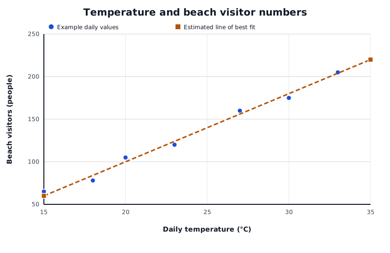
An example of a positive relationship. The line summarises the pattern rather than connecting individual observations.
Data for Temperature and beach visitor numbers
| Series | Daily temperature (°C) | Beach visitors (people) |
|---|---|---|
| Example daily values | 15 | 65 |
| Example daily values | 18 | 78 |
| Example daily values | 20 | 105 |
| Example daily values | 23 | 120 |
| Example daily values | 27 | 160 |
| Example daily values | 30 | 175 |
| Example daily values | 33 | 205 |
| Example daily values | 35 | 220 |
| Estimated line of best fit | 15 | 60 |
| Estimated line of best fit | 35 | 220 |
The points show a strong positive relationship: warmer days generally have more visitors. The scatter means that temperature alone would not give an exact visitor count. Different days could also differ in rainfall, holidays or transport availability.
A trend line summarises the overall direction of the points. An estimated line of best fit represents the pattern and can be used to make predictions.
For a roughly straight pattern, place your ruler on the graph on its edge. Move it until it follows the shape of the data, with roughly the same number of points above and below it. Ignore points lying on the line when counting. Draw a single straight line across the data range, stopping at the first and last plotted points. It need not pass through any particular observation.
Where the points closely follow a curved pattern, sketch a smooth curve that follows them. This suggests a possible non-linear relationship: the pattern is curved rather than straight.
To predict a visitor count from the plotted line, locate the temperature on the horizontal axis, move vertically to the line, then horizontally to the visitor axis. At 25°C, this line gives about 140 visitors. This is an estimate of the general pattern, not a guarantee for an individual day.
A line graph commonly shows how a variable changes over time, with successive observations connected in time order. It can help estimate values between observations or predict what might happen later.
Interpolation estimates within the available data range. Extrapolation extends a trend beyond that range.
Suppose a town has the following population figures: 10,000 in 2020, 12,000 in 2022 and 14,000 in 2024. The graph also shows what continuing the same trend would imply.
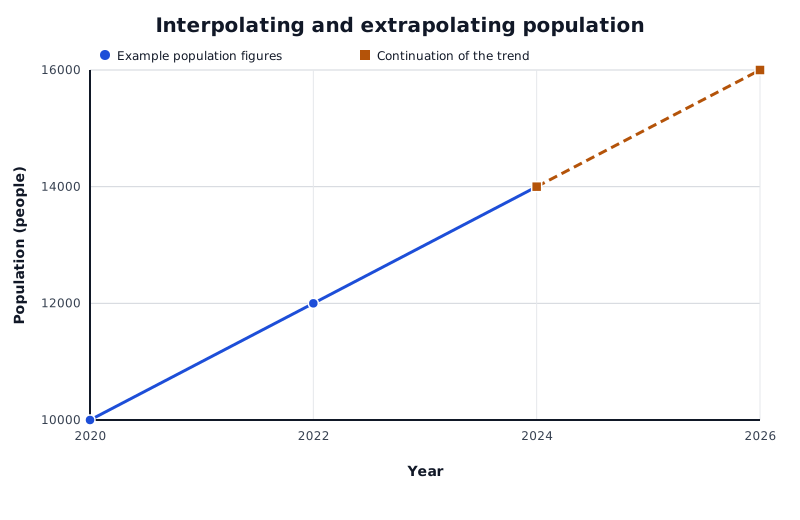
Suppose a town's population follows this pattern. Estimates between 2020 and 2024 are interpolation; extending the trend beyond 2024 is extrapolation.
Data for Interpolating and extrapolating population
| Series | Year | Population (people) |
|---|---|---|
| Example population figures | 2020 | 10000 |
| Example population figures | 2022 | 12000 |
| Example population figures | 2024 | 14000 |
| Continuation of the trend | 2024 | 14000 |
| Continuation of the trend | 2026 | 16000 |
To interpolate for 2023, move up from 2023 to the line between the 2022 and 2024 observations, then across to the population axis. Halfway between 12,000 and 14,000 gives an estimate of 13,000 people. This assumes that change between those observations was approximately steady.
To extrapolate to 2026, continue the recent trend beyond 2024. An increase of 2,000 people every two years would suggest 16,000 people in 2026. This is a conditional prediction: it depends on that rate continuing. Changes in migration, housing provision or employment could alter the trend.
Interpolation is generally more dependable than extrapolation because it stays within the range of evidence. Neither is automatically accurate. Widely spaced observations, irregular changes or a weak relationship reduce confidence in a prediction.
A graph can be accurately drawn yet support a misleading conclusion if the displayed data are selective. Suppose a visitor survey includes only sunny weekend days. Its relationship between temperature and visitor numbers may not represent wet weekdays or the whole year. Presenting it as evidence for all days would extend the conclusion beyond the sample.
Cherry-picking means displaying data that support a particular claim while leaving out data that challenge it. Displaying only points close to a trend and omitting other observations could make a scatter plot's relationship appear stronger than the complete data justify. Selecting a short period can also change the apparent direction of a trend: a temporary fall may occur within a longer-term rise. Compare the conclusion with the number, range and selection of observations. Ask which places, groups or periods are missing and whether those omissions matter.
Axis scales affect the visual impression too. Suppose a line graph shows a population rising from 10,000 to 10,200. A vertical scale from 0 to 20,000 makes the rise look small; a scale from 9,900 to 10,300 makes the same rise look much larger. The numerical change remains 200 people. A restricted scale is not automatically wrong, but judging change from the line's appearance alone could be misleading. Read the axis labels, units and intervals, then compare the actual values.
A small sample provides limited evidence. A sample drawn from only one place or group may also be unrepresentative, even if its points show a strong relationship. Greater scatter around a line makes individual predictions less certain, while extrapolation adds the risk that the pattern will change outside the observed range.
Finally, correlation does not prove causation. Two variables varying together does not establish that one causes the other. A positive relationship between temperature and beach visitors is consistent with warm weather encouraging visits, but holidays and other conditions may also influence attendance.
A justified conclusion describes the relationship shown, acknowledges the sample's limits and avoids claiming more than the evidence supports. For the beach example, it would be reasonable to conclude that warmer days tend to have more visitors in the displayed sample. It would not be reasonable to claim that temperature alone determines attendance on every day of the year.
Describe a relationship using both variable names, its direction and its strength; support your description with values from the graph.
Draw an estimated line of best fit through the middle of the scatter, not by joining successive points or forcing it through the origin.
State whether a prediction is interpolation or extrapolation and explain its reliability in the context of the data.
A limitation needs a consequence: explain how a small or selective sample could make the conclusion unrepresentative.
Check axis scales and the period displayed before judging the size or direction of a change.
Correlation does not prove causation. Suggest a relevant alternative influence rather than simply repeating this phrase.
It can see this note and what your specification asks for.
Answers are free with an account.
1 free note left this week
Get more free notesYour answer sets when this note comes back for review, or marks it complete.
Was this note helpful?
Log in to tell us whether it helped, or to report a problem.
Last updated
Bivariate data
Data recording two variables for each observation, such as temperature and visitor numbers on each day.
Correlation
A relationship between two variables: positive when they tend to increase together, and negative when one tends to decrease as the other increases.
Line of best fit
A line drawn to represent the overall relationship in a scatter plot, rather than passing through every point.
Interpolation
An estimate made within the range covered by the available data.
Extrapolation
An estimate made beyond the range covered by the available data, assuming the trend continues.
Outlier
An observation that lies noticeably away from the main pattern of the data.
Selective statistical presentation
Choosing which data to display or emphasise in a way that may give an incomplete or misleading impression.
Put your knowledge into practice — try past paper questions for Geography A
Bivariate data
Data recording two variables for each observation, such as temperature and visitor numbers on each day.
Correlation
A relationship between two variables: positive when they tend to increase together, and negative when one tends to decrease as the other increases.
Line of best fit
A line drawn to represent the overall relationship in a scatter plot, rather than passing through every point.
Interpolation
An estimate made within the range covered by the available data.
Extrapolation
An estimate made beyond the range covered by the available data, assuming the trend continues.
Outlier
An observation that lies noticeably away from the main pattern of the data.
Selective statistical presentation
Choosing which data to display or emphasise in a way that may give an incomplete or misleading impression.
Check sample size, representativeness, omitted observations, selected dates and axis scales. Cherry-picking can distort the apparent direction or strength of a pattern; scales can exaggerate or minimise apparent change.
Correlation is not proof of causation. Keep conclusions within the evidence and explain why each limitation matters.