

Loading…
Loading…
Loading…
OCR GCSE Geography A · J383
OCR J383 · Data Analysis and Statistics Check the specification (PDF) (opens in a new tab)
A fieldwork survey produces individual observations: sediment lengths, river depths, pedestrian counts or questionnaire answers. To compare places, geographers often need a summary of these observations. Measures of central tendency describe a typical value, while measures of spread describe how much the values vary.
These summaries answer different questions. Two beaches might have the same typical sediment size but very different mixtures of small and large particles. A useful comparison therefore often combines a measure of central tendency with a measure of spread.
The mean uses every value. Add the measurements, then divide by the number of measurements:
The median is the middle value after putting the data in ascending order, from smallest to largest. For an odd number of values, there is one middle value. For an even number, add the two middle values and divide by two.
The mode is the most frequent value. There may be more than one mode, or no mode if every value occurs equally often. Unlike the mean, the mode can also summarise categories, such as the most frequently reported method of travelling to school.
Choosing a summary depends on the data. The mean includes all measurements but can be pulled upwards or downwards by an unusually extreme value. The median is less affected by extremes, so it can better represent a typical value in an uneven dataset. The mode identifies what occurs most often, but does not describe the whole distribution.
Before calculating, read the title, column headings and units. Check what each row represents and whether the table includes summary rows. A row containing a mean is not an extra observation.
The following measurements are sediment lengths along axis a, in centimetres, from two locations in Saundersfoot Bay. Each numbered row contains one measurement from each location; the rows are ordered by size, not by distance along the beach.
| Measurement number | Location A: length (cm) | Location B: length (cm) |
|---|---|---|
| 1 | 5.2 | 6.2 |
| 2 | 7.6 | 6.2 |
| 3 | 8.8 | 6.3 |
| 4 | 9.3 | 6.5 |
| 5 | 9.8 | 8.3 |
| 6 | 11.4 | 8.8 |
| 7 | 11.8 | 9.2 |
| 8 | 12.6 | 10.1 |
| 9 | 13.9 | 11.3 |
| 10 | 18.1 | 13.2 |
| 11 | 21.5 | 14.6 |
There are 11 measurements at each location, so the median is the sixth value: 11.4 cm at A and 8.8 cm at B. Location A therefore has a larger median sediment length. At B, 6.2 cm occurs twice and every other value once, making 6.2 cm the mode. A has no mode.
To calculate B's mean, add its 11 lengths to obtain 100.7 cm, then divide by 11. The mean is approximately 9.15 cm. This is slightly larger than its median of 8.8 cm because the larger measurements affect the mean.
A table comparison should identify the quantity being compared and support it with values. Here, larger typical sediment lengths at A do not mean that every particle measured at A is larger than every particle at B.
The range measures the full span of the data:
At A, the range is cm. At B, it is cm. The complete set of lengths is therefore more spread out at A. However, the range depends only on the two extreme measurements.
The interquartile range, or IQR, measures the spread of the middle 50% instead. The lower , , marks approximately one-quarter of the ordered data; the upper quartile, , marks approximately three-quarters.
For an ordered list containing measurements, the quartile rank positions used here are:
With 11 measurements, these positions are the third and ninth values. At A, the lower quartile is 8.8 cm and the upper quartile is 13.9 cm. At B, they are 6.3 cm and 11.3 cm.
The IQR is therefore 5.1 cm at A and 5.0 cm at B. Although A has a much larger overall range, the spread of the middle half of the measurements is very similar at the two locations. IQR is a measure of spread, not central tendency, and is less affected by extreme values than the range.
Large datasets are often grouped into intervals. The frequency is the number of observations in each interval. The modal class is the interval with the greatest frequency: it identifies the most common group, not an exact measurement within it.
Suppose a sediment survey records 40 particle lengths and groups them as follows:
| Sediment length, (cm) | Frequency | Cumulative frequency |
|---|---|---|
| 4 | 4 | |
| 8 | 12 |
The modal class is cm, with 12 particles. To obtain cumulative frequency, keep adding the frequencies: the total up to 4 cm is , and the total up to 6 cm is 20. The final cumulative frequency equals the sample size, 40.
A cumulative frequency graph plots the upper class boundaries against these running totals. Begin at the lower boundary with a cumulative frequency of zero. The graph never falls because observations are being added, not removed.
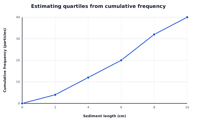
Suppose a survey records 40 sediment lengths. Read across from cumulative frequencies 10, 20 and 30 to estimate the lower quartile, median and upper quartile.
Data for Estimating quartiles from cumulative frequency
| Series | Sediment length (cm) | Cumulative frequency (particles) |
|---|---|---|
| Cumulative number of particles | 0 | 0 |
| Cumulative number of particles | 2 | 4 |
| Cumulative number of particles | 4 | 12 |
| Cumulative number of particles | 6 | 20 |
| Cumulative number of particles | 8 | 32 |
| Cumulative number of particles | 10 | 40 |
To estimate the median from this graph, find half the total frequency: . Read horizontally from 20 on the cumulative frequency axis to the plotted line, then vertically down to the length axis. The estimated median is 6 cm.
For the lower quartile, use on the cumulative frequency axis; for the upper quartile, use . Reading across and down gives approximately 3.5 cm and 7.7 cm. Their difference gives an estimated IQR of about 4.2 cm.
These graph readings are estimates because grouping hides individual measurements. The connected points assume a steady accumulation within each interval. On an actual cumulative frequency diagram, follow its plotted line or curve and use its scales. The , and graph-reading levels are distinct from the rank-position calculations used for a raw list.
Good analysis begins before fieldwork. Design the sheet around the question and the measurements needed to answer it. Include a clear investigation title, site identifiers, location, date, time, recorder and relevant conditions. Put units in column headings and provide space for repeated measurements and site notes.
For a river investigation, a useful sheet could have a site summary recording site ID, location, channel width (m), date, time and conditions. A depth table for each site could use the headings distance from starting bank (m) and depth (m), with one row for every measurement across the channel. A separate table could record repeated flow measurements, with the appropriate units. Recording each measurement's position makes it possible to draw a cross-section later.
An investigation of downstream change on the River Tillingbourne illustrates why these details matter. Units in headings make measurements clear; site notes support descriptions; repeated flow measurements allow an average. Inconsistent decimal places make depth records harder to compare, while missing distances between depth measurements prevent their positions being reconstructed. Photographs can help explain local conditions, but cannot replace the measurements needed for a cross-section.
Test the sheet before the main survey. Check that another person understands the headings and that there is enough space for every planned measurement. Collection is complete when the planned sites, measurements and repeats have been recorded, with notes explaining any missing data.
Accuracy means closeness to the true value. Read instruments carefully, use suitable equipment and check that measurements are recorded in the correct units. For pedestrian counts, agree exactly what counts as a crossing so that people are not missed or counted twice. Record measurements to a consistent precision appropriate to the instrument; extra decimal places do not automatically make a reading more accurate.
Reliability concerns consistency when the method is repeated under comparable conditions. Use the same equipment, definitions and procedures at different sites. Repeat measurements so that variation can be assessed and an average calculated. Repeating an incorrect method can give consistent but inaccurate results.
The sample size is the number of observations collected. It must be large enough, and sufficiently well distributed, to represent the variation relevant to the question. Surveying many people in just one place or at one time may still miss important groups. There is no single sample size suitable for every investigation.
Systematic sampling collects data at regular intervals. For example, a litter investigation in Sheffield used sites along a transect from the train station towards the city centre. A transect is a line across an area along which observations can reveal change. Regular intervals make site selection repeatable, although one transect may not represent the whole city.
A control group provides a comparison without the factor being investigated. For example, to investigate a litter-reduction campaign, compare an area receiving the campaign with a similar area not receiving it. Use the same counting method, survey area and timing in both. Differences in footfall or land use could otherwise affect the comparison. A control is useful where the investigation calls for one; it is not required for every descriptive survey.
Plan only measurements that can be collected safely. For river work, follow the teacher's risk assessment, use approved access points and avoid deep or fast-flowing water and unstable banks. For street surveys, work from a safe pavement position without obstructing pedestrians, and avoid recording identifying personal information. Record an unsafe or inaccessible site as missing rather than taking a risk or inventing a result.
Put raw data in ascending order before finding the median or quartiles. A quartile's rank position is not its measured value.
For an even number of observations, average the two middle values to find the median.
Keep measurement units in your answers: a range or interquartile range of sediment lengths is measured in cm, not cm².
Distinguish a modal class, which is an interval, from a mode, which is an individual value.
On a cumulative frequency graph, read across from the required cumulative frequency, then down to the measurement axis.
Explain a fieldwork improvement precisely: say what you would change and how it would improve the data. A larger sample alone does not remove bias.
It can see this note and what your specification asks for.
Answers are free with an account.
1 free note left this week
Get more free notesYour answer sets when this note comes back for review, or marks it complete.
Was this note helpful?
Log in to tell us whether it helped, or to report a problem.
Last updated
Central tendency
A statistic describing the centre or typical value of a dataset, such as the mean, median or mode.
Mean
The sum of all measured values divided by the number of values.
Median
The middle value in an ordered dataset; with an even number of values, the average of the two middle values.
Mode
The value occurring most frequently in a dataset.
Modal class
The class interval containing the greatest frequency in a grouped frequency table.
Spread
The extent to which values in a dataset vary, measured using statistics such as the range or interquartile range.
Range
The largest value minus the smallest value in a dataset.
Quartile
One of the values dividing ordered data into four parts. The lower quartile marks approximately 25% of the data and the upper quartile approximately 75%.
Interquartile range
The upper quartile minus the lower quartile, measuring the spread of the middle 50% of the data: .
Cumulative frequency
A running total of frequencies up to a particular value or class boundary.
Accuracy
How close a measurement or count is to the true value.
Sample size
The number of observations, measurements or people included in a sample.
Reliability
The extent to which a method produces consistent results when repeated under comparable conditions.
Representative sample
A sample reflecting the relevant characteristics and variation of the wider population or area being investigated.
Systematic sampling
Collecting observations at regular intervals, such as every 10 m along a survey route.
Bias
An unfair influence on how data are selected, collected or interpreted, which can distort the results.
Control group
A comparison group not exposed to the factor being investigated, while other relevant conditions are kept as similar as possible.
Put your knowledge into practice — try past paper questions for Geography A
Central tendency
A statistic describing the centre or typical value of a dataset, such as the mean, median or mode.
Mean
The sum of all measured values divided by the number of values.
Median
The middle value in an ordered dataset; with an even number of values, the average of the two middle values.
Mode
The value occurring most frequently in a dataset.
Modal class
The class interval containing the greatest frequency in a grouped frequency table.
Spread
The extent to which values in a dataset vary, measured using statistics such as the range or interquartile range.
Range
The largest value minus the smallest value in a dataset.
Quartile
One of the values dividing ordered data into four parts. The lower quartile marks approximately 25% of the data and the upper quartile approximately 75%.
Interquartile range
The upper quartile minus the lower quartile, measuring the spread of the middle 50% of the data: .
Cumulative frequency
A running total of frequencies up to a particular value or class boundary.
Accuracy
How close a measurement or count is to the true value.
Sample size
The number of observations, measurements or people included in a sample.
Reliability
The extent to which a method produces consistent results when repeated under comparable conditions.
Representative sample
A sample reflecting the relevant characteristics and variation of the wider population or area being investigated.
Systematic sampling
Collecting observations at regular intervals, such as every 10 m along a survey route.
Bias
An unfair influence on how data are selected, collected or interpreted, which can distort the results.
Control group
A comparison group not exposed to the factor being investigated, while other relevant conditions are kept as similar as possible.
| 8 | 20 |
| 12 | 32 |
| 8 | 40 |
For an ascending raw list, quartile positions used here are and .
Add frequencies progressively. The final total is the sample size, .
On a cumulative frequency graph, read across to the line or curve and down to the measurement axis from:
Grouped-data readings are estimates.
Check headings, units, intervals and totals. Distinguish observations from summary rows. Compare like with like and support a pattern with values.
Saundersfoot Bay: median lengths A 11.4 cm, B 8.8 cm; ranges A 16.3 cm, B 8.4 cm; IQRs A 5.1 cm, B 5.0 cm. A has a larger median and overall range, but almost the same middle-half spread.