

Loading…
Loading…
Loading…
OCR GCSE Geography A · J383
OCR J383 · Data Analysis and Statistics Check the specification (PDF) (opens in a new tab)
Geographers often investigate whether two things vary together. For example, does noise level decrease with distance from a busy road? Bivariate data consists of paired values for two variables. Each pair must refer to the same observation: the distance and noise level recorded at one survey site belong together.
A scatter plot displays these pairs. One variable goes on the horizontal axis and the other on the vertical axis. Label both axes with the variable and its unit, choose evenly spaced numerical scales and plot each pair as a separate point. Unlike a line graph showing change over time, the individual points are not joined together.
Correlation describes how two variables vary together. Read the pattern from left to right:
Direction and strength are different. Points clustered closely around a clear trend show stronger correlation than points scattered widely around it. A steep slope does not necessarily mean strong correlation: strength depends on how closely the points follow the pattern.
Suppose a survey produced the following noise levels at eight sites near a road. The horizontal axis shows distance in kilometres; the vertical axis shows noise level in decibels, written dB.
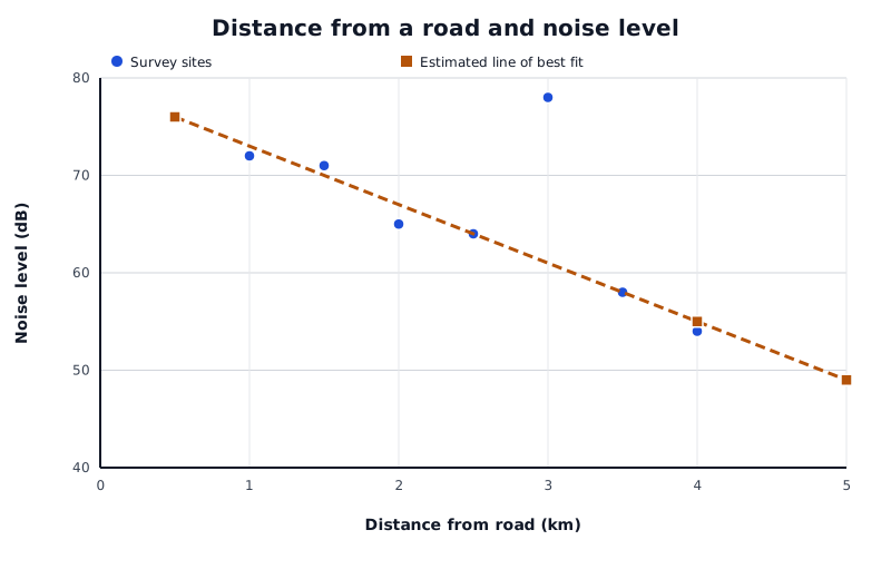
Suppose these readings were collected near a road. Most show decreasing noise with distance, but one site lies well above the main trend. The estimated line extends beyond the observed distances to demonstrate extrapolation.
Data for Distance from a road and noise level
| Series | Distance from road (km) | Noise level (dB) |
|---|---|---|
| Survey sites | 0.5 | 76 |
| Survey sites | 1 | 72 |
| Survey sites | 1.5 | 71 |
| Survey sites | 2 | 65 |
| Survey sites | 2.5 | 64 |
| Survey sites | 3 | 78 |
| Survey sites | 3.5 | 58 |
| Survey sites | 4 | 54 |
| Estimated line of best fit | 0.5 | 76 |
| Estimated line of best fit | 4 | 55 |
| Estimated line of best fit | 5 | 49 |
The main pattern is negative correlation: sites farther from the road generally have lower noise levels. At 0.5 km, the noise level is 76 dB; at 4 km, it is 54 dB. However, the site at 3 km has a noise level of 78 dB and lies well above the main pattern. This is an outlier. A nearby noise source or a measurement problem could explain it, but the graph alone cannot tell us which.
A trend line summarises the overall direction of the points. Begin by looking at the main cluster and sketching its general trend. Where the pattern is roughly straight, draw an estimated straight line of best fit with a ruler.
Place it through the centre of the main cluster, with roughly balanced numbers of points and distances on either side. It need not pass through particular points. Do not let a single outlier pull it away from the main pattern, and do not force it through the origin unless the data and context justify that choice.
The line in the noise example represents the overall decrease rather than every individual site's reading. If there is no clear relationship, a straight line will not provide a useful prediction.
To estimate noise level at a given distance, find the distance on the horizontal axis, move vertically to the line of best fit, then move horizontally to the vertical axis. Read the estimated noise level, including its unit.
For a distance of 2.25 km, the example line gives approximately 66 dB. This is interpolation, because 2.25 km lies within the observed distance range of 0.5–4 km. It estimates the general pattern, not the exact reading guaranteed at a particular site.
Extending the line to 5 km gives approximately 49 dB. This is extrapolation, because 5 km lies beyond the observed range. It is less reliable: the relationship may change farther from the road, or other noise sources may become more important. A larger, appropriately collected sample and a clearer relationship generally provide a firmer basis for predictions, but neither makes them certain.
Before accepting a graph's message, check its title, labels, units, scale and any key. These tell you what is being compared and how values should be read.
Equal distances along an ordinary numerical axis should represent equal changes in value. For example, labels of 0, 10, 20 and 50 at equal intervals would distort the graph. A missing key on a graph containing two groups prevents you from identifying their results. Missing units make numerical values ambiguous.
An axis starting above zero is not automatically incorrect, but it can make differences appear larger. Read the actual values rather than judging only the visual height or spacing. Likewise, check whether two graphs use the same scale before comparing their appearance.
Also distinguish weaknesses in presentation from limitations in the evidence. A neatly labelled graph can still represent a small sample or measurements made under different conditions. Those limitations affect how confidently its findings can be applied more widely.
A useful conclusion connects a claim to numerical evidence and explains its geographical meaning. For the example, you could conclude: ‘The data generally support a decrease in noise level with distance from the road: readings fall from 76 dB at 0.5 km to 54 dB at 4 km. However, the 78 dB reading at 3 km shows that distance alone does not explain every site's noise level.’
When comparing groups, use appropriate averages and measures of spread. A higher median indicates a higher typical value; a larger range or interquartile range indicates greater variation. Give the figures and explain them in context, rather than simply listing statistics. Comparisons are more convincing when the measurements were taken using comparable procedures and conditions.
Finally, correlation does not establish causation. Two variables may vary together because another factor influences both. Sunflower height and puppy weight, for example, may both increase with time, but one does not cause the other. A scatter plot supports a statement about an observed relationship; establishing its cause requires further evidence.
Draw an estimated line through the centre of the main pattern, balancing points and distances on either side.
Read from the known axis value to the line, then across to the other axis.
Describe a relationship using both variables: ‘As distance from the road increases, noise level generally decreases’, rather than just ‘negative correlation’.
Draw a line of best fit through the centre of the main cluster, not by joining the points or forcing the line through the origin.
Identify an outlier, but do not assume it is a recording error. It may represent a genuine local difference.
Support conclusions with figures and units, then explain what those figures mean geographically.
When identifying a weakness, explain its effect: a missing key prevents the reader from identifying which dataset each symbol represents.
It can see this note and what your specification asks for.
Answers are free with an account.
1 free note left this week
Get more free notesYour answer sets when this note comes back for review, or marks it complete.
Was this note helpful?
Log in to tell us whether it helped, or to report a problem.
Last updated
Bivariate data
Data containing paired values for two variables, such as distance from a road and noise level at each survey site.
Scatter plot
A graph in which each point represents a pair of numerical values, allowing a relationship between two variables to be examined.
Correlation
A pattern describing how two variables vary together. Correlation alone does not establish that one variable causes changes in the other.
Positive correlation
A relationship in which one variable generally increases as the other increases.
Negative correlation
A relationship in which one variable generally decreases as the other increases.
Line of best fit
An estimated line through the centre of a scatter plot's main pattern, used to summarise the relationship and make predictions.
Interpolation
Estimating a value within the range of the available data.
Extrapolation
Estimating a value beyond the range of the available data by extending an existing trend.
Outlier
A data value that lies well away from the general pattern of the other values.
Put your knowledge into practice — try past paper questions for Geography A
Bivariate data
Data containing paired values for two variables, such as distance from a road and noise level at each survey site.
Scatter plot
A graph in which each point represents a pair of numerical values, allowing a relationship between two variables to be examined.
Correlation
A pattern describing how two variables vary together. Correlation alone does not establish that one variable causes changes in the other.
Positive correlation
A relationship in which one variable generally increases as the other increases.
Negative correlation
A relationship in which one variable generally decreases as the other increases.
Line of best fit
An estimated line through the centre of a scatter plot's main pattern, used to summarise the relationship and make predictions.
Interpolation
Estimating a value within the range of the available data.
Extrapolation
Estimating a value beyond the range of the available data by extending an existing trend.
Outlier
A data value that lies well away from the general pattern of the other values.
Check labels, units, keys and numerical scales. Distinguish misleading presentation from limitations such as small samples or inconsistent measurement conditions.
Build a conclusion from claim → figures with units → geographical meaning → relevant qualification. When comparing groups, consider both typical values and variation.