

Loading…
Loading…
Loading…
Eduqas GCSE Geography B · C112
Eduqas C112 · 4.1 Graph Construction and Selection Check the specification (PDF) (opens in a new tab)
Select and construct appropriate charts and graphs using accurate scales to present geographical data.
Create bar charts, line charts, climate graphs, and hydrographs to represent temporal and continuous data.
Construct pie charts, pictograms, and proportional circles to display categorical data proportions.
Develop histograms with equal class intervals, dispersion graphs, and scatter graphs to analyze distributions.
Construct specialized geographical graphics including star graphs, radial graphs, kite diagrams, and triangular graphs.
Geographers choose graphs according to the question they want to investigate. A histogram shows how frequently values occur within numerical groups. A dispersion graph keeps the individual values visible, showing how closely grouped or widely spread they are. Both can represent one variable, such as pebble size. A scatter graph has a different purpose: it investigates a relationship between two variables, such as traffic counts and noise levels.
Before drawing any of these graphs, identify the variable or variables, their units and the smallest and largest values. Choose scales that accommodate the data and make differences easy to read. Equal distances along a numerical axis must represent equal changes in value.
Continuous data can take any value within a range. For example, a pebble's length might be 4 cm, 4.3 cm or 4.35 cm, depending on the precision of the measurement. A histogram groups these measurements into class intervals and shows the , or number of observations, in each interval.
For this technique, use class intervals of equal width. Suppose a sample of 20 pebbles has the following lengths, grouped into intervals 2 cm wide:
| Pebble length (cm) | Frequency |
|---|---|
| 0 to less than 2 | 2 |
| 2 to less than 4 | 4 |
| 4 to less than 6 | 7 |
| 6 to less than 8 | 5 |
| 8 to less than 10 | 2 |
The boundaries prevent double counting: a pebble exactly 4 cm long belongs in the 4 to less than 6 cm interval, not the preceding one.
To construct the histogram, label the horizontal axis Pebble length (cm) and mark the boundaries 0, 2, 4, 6, 8 and 10 at equal spacings. Label the vertical axis Frequency and use a scale starting at zero that reaches at least 7. Draw each bar across its entire class interval, with its height equal to the frequency. The bars touch because the length scale is continuous; these are not separate categories.
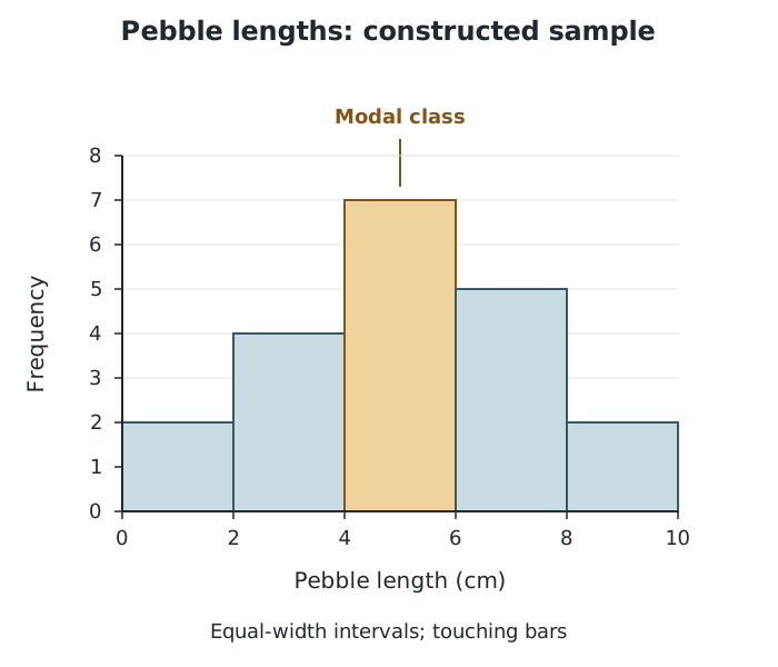
Each bar spans a 2 cm interval; its height shows how many pebbles fall within it.
The tallest bar identifies the modal class: 4 to less than 6 cm, containing seven pebbles. There are 12 pebbles between 4 cm and less than 8 cm, so this is where most of the sample is concentrated. However, the histogram does not reveal their exact individual lengths.
The overall shape also matters. An approximately bell-shaped distribution, balanced around its centre, suggests a normal distribution. An uneven distribution with a longer tail towards one end is skewed. Describe the whole pattern rather than judging its shape from the tallest bar alone.
A dispersion graph plots every observation along a numerical scale. It is useful when an enquiry needs to compare variation within samples, such as pebble sizes at different points on a beach.
Suppose a sample contains pebble sizes of 18, 19, 20, 22, 24, 25, 26, 28, 31, 33 and 34 mm. Draw a vertical axis labelled Pebble size (mm), with a scale covering all these values. Above a sample label, plot one small cross at the height of each measurement. All the crosses belong to the same sample column; horizontal position is not a second measured variable. If a value occurs more than once, place the marks beside one another at the same height so that no observations disappear.
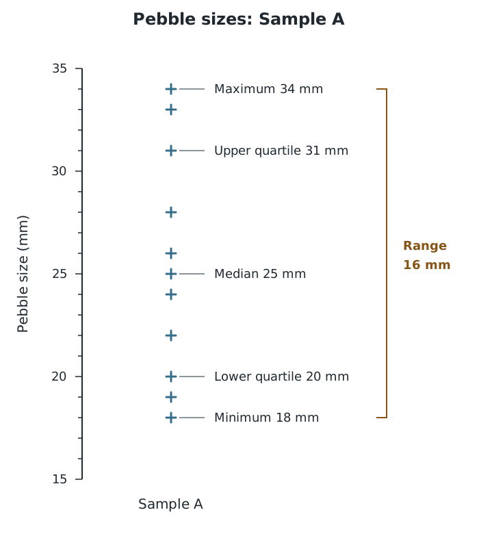
Individual points reveal the sample's spread, including its minimum, maximum and middle value.
The lowest point is 18 mm and the highest is 34 mm. Their difference gives the range:
This means the sample spans 16 mm from its smallest to its largest pebble. The gaps and clusters also show how the values are distributed within that span.
Ordering the values helps identify the middle of the sample. Here, the sixth of the 11 values is the median, 25 mm. The lower and upper quartiles are 20 mm and 31 mm, giving an interquartile range of 11 mm. Unlike the full range, this describes the spread of the middle half of the data.
To compare samples, draw a separate column for each on the same vertical scale. A more tightly grouped column suggests more similar pebble sizes; a wider spread suggests greater variation. This can help investigate sediment sorting, although the graph alone does not explain what caused the differences.
A scatter graph needs two measurements for each observation. For example, an enquiry might record both distance from an urban centre and noise level at each site. Each point represents one site's pair of measurements.
Put the independent variable, used to investigate possible changes in the other variable, on the horizontal axis. Put the dependent variable, whose variation is being investigated, on the vertical axis. Here, distance goes horizontally and noise level vertically. In an enquiry comparing countries' gross national income, or GNI, with infant mortality, GNI would go horizontally and infant mortality vertically.
Suppose five sites have these distance and noise-level pairs: (0 m, 64 dB), (100 m, 57 dB), (200 m, 43 dB), (300 m, 37 dB) and (400 m, 24 dB). Choose a distance scale covering 0–400 m and a noise scale covering 0–70 dB. For the point (200, 43), locate 200 m horizontally, then 43 dB vertically, and mark their intersection. Repeat for every pair without joining the points.
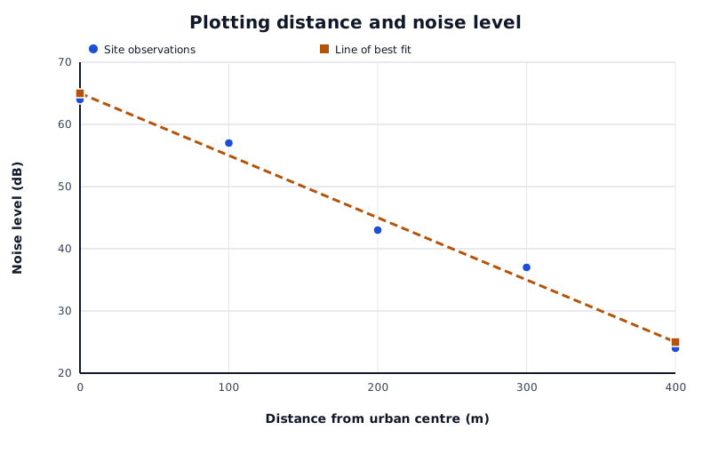
In this constructed example, noise level generally decreases as distance increases. The line follows the trend rather than joining the observations.
Data for Plotting distance and noise level
| Series | Distance from urban centre (m) | Noise level (dB) |
|---|---|---|
| Site observations | 0 | 64 |
| Site observations | 100 | 57 |
| Site observations | 200 | 43 |
| Site observations | 300 | 37 |
| Site observations | 400 | 24 |
| Line of best fit | 0 | 65 |
| Line of best fit | 400 | 25 |
Read the pattern from left to right:
This example shows negative correlation: noise levels tend to be lower farther from the centre. A line of best fit represents that overall trend. Draw it through the middle of the point pattern, aiming for approximately equal numbers of points above and below it rather than connecting individual points.
Points close to the line suggest a strong relationship; widely scattered points suggest a weaker one. A scatter graph gives a visual judgement, not an exact numerical measure of strength. Its appearance also depends on the axis scales and proportions. Finally, an association does not by itself establish cause: explaining a geographical relationship requires evidence about the processes involved.
Label numerical axes with the variable and its unit, and use equal numerical steps for equal distances along each axis.
For an equal-class-interval histogram, plot class boundaries rather than class midpoints. Bars touch, and their heights show frequencies.
Keep every observation when drawing a dispersion graph, including repeated values.
On a scatter graph, plot paired values from the same observation. Do not sort the two variables separately.
A line of best fit follows the overall trend; it does not join successive points or have to pass through every point.
It can see this note and what your specification asks for.
Answers are free with an account.
1 free note left this week
Get more free notesYour answer sets when this note comes back for review, or marks it complete.
Was this note helpful?
Log in to tell us whether it helped, or to report a problem.
Last updated
Histogram
A graph showing the frequency distribution of continuous data grouped into class intervals, with touching bars.
Class interval
A numerical group with a lower and upper boundary, such as lengths from 4 cm up to but not including 6 cm.
Frequency
The number of observations with a particular value or within a particular class interval.
Modal class
The class interval containing the greatest number of observations.
Dispersion graph
A graph plotting each individual value in a dataset along a numerical scale to show its distribution and spread.
Range
The difference between the largest and smallest values in a dataset: .
Scatter graph
A graph in which each point represents a pair of values, used to investigate the relationship between two variables.
Correlation
A pattern of association between two variables, which may be positive, negative or absent.
Line of best fit
A line drawn through a scatter graph to represent the general trend, with approximately equal numbers of points on either side.
Put your knowledge into practice — try past paper questions for Geography B
Histogram
A graph showing the frequency distribution of continuous data grouped into class intervals, with touching bars.
Class interval
A numerical group with a lower and upper boundary, such as lengths from 4 cm up to but not including 6 cm.
Frequency
The number of observations with a particular value or within a particular class interval.
Modal class
The class interval containing the greatest number of observations.
Dispersion graph
A graph plotting each individual value in a dataset along a numerical scale to show its distribution and spread.
Range
The difference between the largest and smallest values in a dataset: .
Scatter graph
A graph in which each point represents a pair of values, used to investigate the relationship between two variables.
Correlation
A pattern of association between two variables, which may be positive, negative or absent.
Line of best fit
A line drawn through a scatter graph to represent the general trend, with approximately equal numbers of points on either side.
Histogram: class boundaries on the horizontal axis; frequency on the vertical axis. Bars span the intervals and touch. The tallest bar is the modal class.
Dispersion graph: one mark per observation along a numerical scale. Use separate columns and a shared scale to compare samples. Retain repeated values.
Scatter graph: independent variable horizontally; dependent variable vertically. Plot each paired observation at its coordinate intersection.
A line of best fit follows the overall trend with approximately balanced numbers of points on either side. Closer points suggest stronger correlation. Correlation alone does not establish cause.