

Loading…
Loading…
Loading…
Eduqas GCSE Geography B · C112
Eduqas C112 · 4.1 Graph Construction and Selection Check the specification (PDF) (opens in a new tab)
Select and construct appropriate charts and graphs using accurate scales to present geographical data.
Create bar charts, line charts, climate graphs, and hydrographs to represent temporal and continuous data.
Construct pie charts, pictograms, and proportional circles to display categorical data proportions.
Develop histograms with equal class intervals, dispersion graphs, and scatter graphs to analyze distributions.
Construct specialized geographical graphics including star graphs, radial graphs, kite diagrams, and triangular graphs.
A useful geographical graph makes the important feature of the data easy to see. Some investigations compare several characteristics of places; others examine direction, changes along a line, or the composition of a whole. These need different graphical arrangements.
Star and radial graphs organise values around a centre. Kite diagrams organise observations along a measured distance. Triangular graphs show how a whole is divided between three components. Whichever you choose, give the graph a descriptive title and label its categories, scales and units.
A star graph, often called a radar graph, has several axes extending from one central point. Each axis represents a different characteristic. Joining the plotted values produces a shape that summarises the dataset.
Suppose two sites have environmental-quality scores for cleanliness, safety, greenery and building condition. Each characteristic is scored from 0 to 5, with higher scores meaning better quality. Site A scores 4, 3, 5 and 2 respectively; Site B scores 2, 4, 3 and 4.
Draw four equally spaced axes from a common centre and label them with the characteristics. Mark 0 at the centre and use equal intervals out to 5 on each axis. Plot Site A's score on each appropriate axis, then join neighbouring points, including the last point back to the first. Repeat for Site B using a different line style and add a key.
The shapes make the contrast visible: Site A scores more highly for cleanliness and greenery, whereas Site B scores more highly for safety and building condition. Use the same category order and scales for both sites. This comparison works because the scores use a shared rating system; unrelated raw measurements should not simply be treated as equivalent scores.
A radial graph represents magnitude by distance from a centre. A directional version, also called a polar graph or rose diagram, places values around the centre according to direction. It is useful for data such as the frequency of winds from different compass directions.
Suppose winds were recorded on 20 occasions: 8 from the north, 6 from the east, 4 from the south and 2 from the west. Draw compass axes with north at the top, east to the right, south at the bottom and west to the left. Mark a common frequency scale from 0 at the centre to 8, using equal intervals.
Draw a spoke along each direction to its recorded frequency: 8 northwards, 6 eastwards, 4 southwards and 2 westwards. Label the scale as the number of observations and give the graph a title explaining that it shows where the winds came from. More detailed datasets can use eight compass directions, provided each observation is assigned consistently.
Unlike the categories on a star graph, these directions have a fixed spatial meaning. The longest spoke identifies the most frequent direction, not the strongest wind: that would require wind-speed data.
A kite diagram shows changes in abundance or frequency along a measured distance, commonly for plant or animal species. Each category has its own horizontal centre line, and the plotted shape is symmetrical above and below it. A wider section represents a larger value.
Suppose equal-sized quadrats are placed at 0, 2, 4, 6 and 8 metres along a transect. Plant A has counts of 0, 4, 8, 2 and 0; Plant B has counts of 0, 0, 2, 6 and 8. The equal sampling areas make these counts comparable.
Draw a horizontal distance axis from 0 to 8 metres and two separate, parallel centre lines, one for each plant. Use the largest count in the whole dataset, 8, to set a common width scale. Using the split-value convention, allow space for 4 count units on either side of each centre line.
At each sampling distance, halve the count and plot that amount above and below the relevant centre line. For example, Plant A's count of 8 at 4 metres is plotted 4 units above and 4 below. A count of 2 is plotted 1 unit on each side; zero lies on the centre line. Join neighbouring points on each side and shade between them.
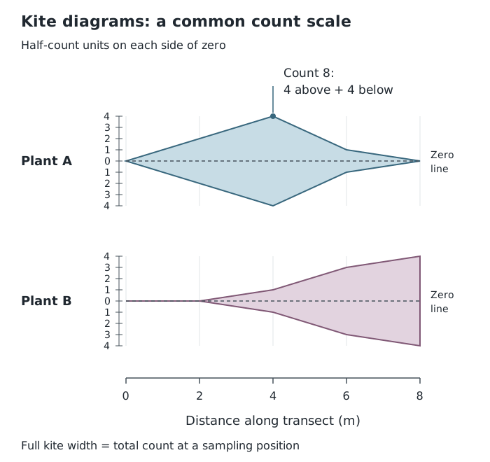
The full kite width represents the count at each sampling position; both plant rows use the same scale.
Label both plant rows, the distance axis and the mirrored count scale. Keep the same scale and row spacing throughout. Plant A reaches its highest count at 4 metres, while Plant B becomes more abundant towards 8 metres. The graph shows this distribution along the sampled line, not across the entire surrounding area. Joining points helps reveal the pattern but does not add observations between sampling positions.
A triangular graph displays three components of a whole. Each component must be expressed as a percentage, and the three percentages must total 100%. It can compare, for example, the proportions of terraced, semi-detached and detached homes in different areas.
Each corner represents 100% of one component and 0% of the other two. The side opposite that corner represents 0% of that component. Moving towards the corner therefore increases its percentage. Lines of equal percentage run parallel to the opposite side.
Suppose Area A contains 50% terraced, 30% semi-detached and 20% detached homes. Draw an equilateral triangle with terraced at the top, semi-detached at the bottom left and detached at the bottom right. Label the percentage scales from 0 to 100, with equal intervals and arrows showing the direction of increase.
Find the 50% terraced line, which runs horizontally, parallel to the base. Then find the 30% semi-detached line, parallel to the triangle's right-hand side. Mark their intersection. Check that the point also lies on the 20% detached line, parallel to the left-hand side.
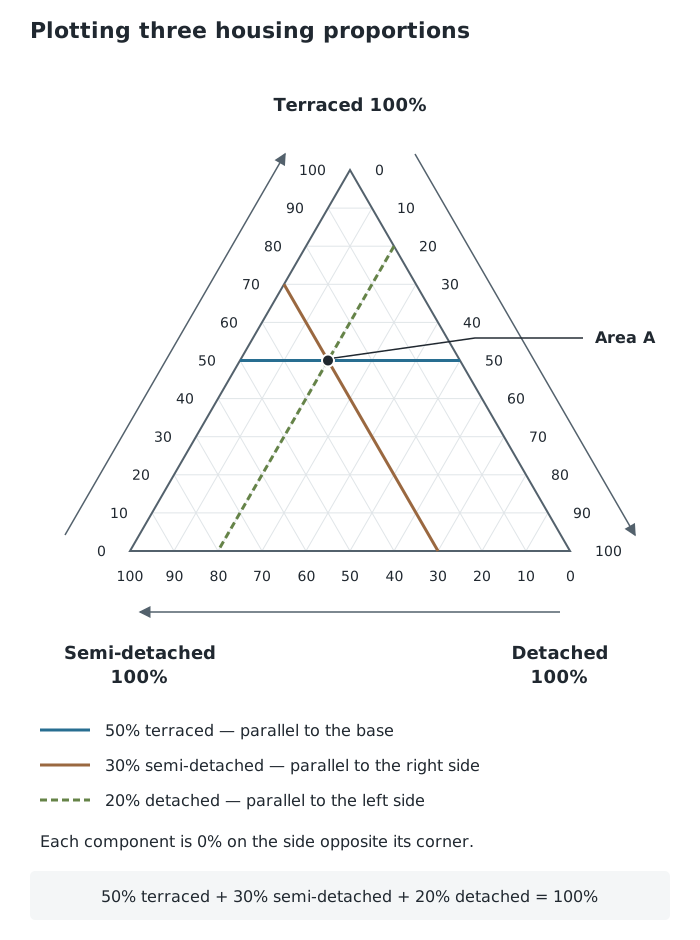
One point represents all three housing proportions. The third percentage checks the intersection.
Two percentages locate the point; the third checks it. Plot each area's complete set of three percentages as one point, using labels or a key to distinguish areas. Nearby points indicate similar compositions. A point closer to the terraced corner indicates a greater terraced proportion, but the graph does not show the total number of homes. On another triangular graph, the corner assignments may differ, so transfer the method by reading its labels and scale directions first.
Star: equally spaced axes → consistent scales → plot each category → join into a closed shape → add a key for comparisons.
Directional radial: label compass directions → use a common scale from the centre → draw each spoke to its value.
Kite: distance on the horizontal axis → separate centre line for each category → common width scale → plot half each value on both sides → join and shade.
Triangular:
Choose the graph to suit the data: several characteristics for a star graph, direction and magnitude for a directional radial graph, changes along a transect for a kite diagram, and three percentage components for a triangular graph.
Label scales, units and categories. Keep scales consistent when comparing sites or categories.
In a kite diagram using the split-value convention, plot half the recorded value on each side of the centre line: the full width represents the total.
For a triangular graph, check that the three percentages total 100%. Follow the labelled scale directions and use lines parallel to the appropriate triangle sides.
It can see this note and what your specification asks for.
Answers are free with an account.
1 free note left this week
Get more free notesYour answer sets when this note comes back for review, or marks it complete.
Was this note helpful?
Log in to tell us whether it helped, or to report a problem.
Last updated
Star graph
A graph with axes radiating from a common centre, used to display several characteristics of a place or dataset. Plotted values are joined to form a shape.
Radial graph
A graph in which distance from a central point represents magnitude. In a directional version, the position around the centre also represents direction.
Kite diagram
A symmetrical graph showing how the abundance or frequency of a category changes along a measured distance.
Transect
A line across an area along which observations or measurements are taken.
Triangular graph
A graph showing the proportions of three components that together make up 100% of a whole.
Put your knowledge into practice — try past paper questions for Geography B
Star graph
A graph with axes radiating from a common centre, used to display several characteristics of a place or dataset. Plotted values are joined to form a shape.
Radial graph
A graph in which distance from a central point represents magnitude. In a directional version, the position around the centre also represents direction.
Kite diagram
A symmetrical graph showing how the abundance or frequency of a category changes along a measured distance.
Transect
A line across an area along which observations or measurements are taken.
Triangular graph
A graph showing the proportions of three components that together make up 100% of a whole.
Label corners and percentage scales. Follow constant-percentage lines parallel to the opposite sides. Plot the intersection of two component lines and check it against the third.
Use matching scales and category arrangements. A kite's width represents abundance, not an area-wide distribution. A triangular graph shows proportions, not totals.