

Loading…
Loading…
Loading…
Eduqas GCSE Geography B · C112
Eduqas C112 · 2.2 Percentages and Percentiles Check the specification (PDF) (opens in a new tab)
Calculate percentage increases and decreases from graphical data, such as population line graphs.
Construct histograms depicting normal and skewed distributions.
Utilize histograms to accurately calculate and interpret percentiles.
Geographical measurements such as rainfall, river depth and sediment size can be grouped into class intervals. A frequency table records how many observations fall within each interval. A histogram turns this table into a picture of the distribution: where observations are concentrated and how widely they are spread.
The horizontal axis shows the measured variable, including its units. Each bar extends from the lower to the upper boundary of its class. Adjacent classes have touching bars because they represent a continuous numerical scale, rather than separate categories.
For example, includes values from 10 up to, but not including, 20. The next class can begin at 20 without counting that value twice.
A histogram represents frequency through bar area. This matters especially when class widths differ: a wider class must not appear to contain more observations merely because its bar is wider.
The height needed is called frequency density:
Since a rectangle’s area is width multiplied by height:
Consider a group of television viewers. Six people watched for between 0 and 100 minutes, while another six watched for between 500 and 800 minutes. Their class widths are 100 and 300 minutes, so their frequency densities are and . The second bar is three times as wide but one-third as high. Both have an area representing six people.
With equal class widths, frequency can be used on the vertical axis because all bar areas have the same proportional relationship to frequency. Using frequency density also works and makes the area calculation consistent across classes.
To draw a histogram, first calculate each class width and, if using a frequency-density axis, each density. Choose evenly spaced numerical scales that accommodate the full range and greatest height. Label both axes, then draw each bar across its actual class boundaries at the appropriate height.
For example, recorded worm lengths were grouped as follows:
| Length, (mm) | Frequency | Class width (mm) | Frequency density (worms per mm) |
|---|---|---|---|
| 6 | 5 | 1.2 | |
| 14 | 10 | 1.4 | |
| 26 | 10 | 2.6 | |
| 2 | 20 | 0.1 |
To plot these data, mark the boundaries 15, 20, 30, 40 and 60 on a length axis. Draw touching bars with heights 1.2, 1.4, 2.6 and 0.1 on a frequency-density axis. The last bar is twice as wide as the preceding one, but much lower: its area represents only two worms.
The completed histogram reveals the shape of the distribution. A normal distribution is symmetrical and bell-shaped: the tallest bars are near the centre, with heights generally decreasing towards both ends. Most observations cluster around the centre, with relatively few very low or very high values. A histogram of sampled measurements may only approximately resemble this shape.
A skewed distribution is not symmetrical. In a positively skewed distribution, most observations are towards the lower end and a long tail extends towards higher values, to the right. In a negatively skewed distribution, most observations are towards the higher end and the long tail extends towards lower values, to the left.
When constructing either shape from a table, plot the given frequencies faithfully. Do not adjust the bars to make a smoother bell or a more obvious tail. With unequal widths, a tall bar indicates a high concentration of observations per unit of the measured variable, not necessarily the largest class frequency.
A percentile identifies a position within an ordered distribution. The 50th percentile is the median: it divides the observations into lower and upper halves. The 90th percentile has approximately 90% of observations below it and 10% above it.
For geographical measurements, a percentile keeps the units of the original variable. For example, the 90th percentile of a set of rainfall measurements is a rainfall amount in millimetres. It is not 90% of the greatest rainfall recorded. Percentiles help identify relatively low or high measurements within a dataset without relying only on its extremes.
On a histogram, frequencies are represented by areas. To find the th percentile, find the point on the horizontal axis with of the total bar area to its left.
A running club recorded 400 m times for 36 members aged under 30. The histogram has four classes: 50–54 seconds, 54–58 seconds, 58–62 seconds and 62–70 seconds. Their frequency densities are 1, 4, 3 and 0.5 members per second.
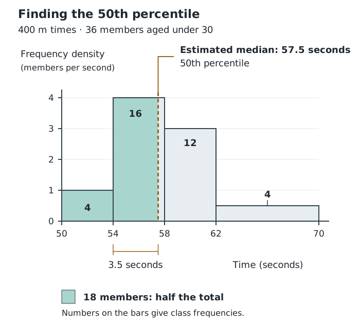
The estimated median divides the total histogram area into two equal parts, each representing 18 members.
Multiplying each width by its density gives frequencies of 4, 16, 12 and 4. Their total is 36. The cumulative frequencies are therefore 4, 20, 32 and 36.
To estimate the 50th percentile, find the value with half the observations below it: . The first class accounts for four observations; the first two account for 20. The required value therefore lies in the 54–58 second class.
After allowing for the first four observations, we need an area representing observations inside this class. Its height is 4, so the required horizontal distance is seconds. Adding this distance to the lower boundary gives seconds. The estimated median time is therefore 57.5 seconds.
The same method applies to other percentiles. First calculate the target cumulative frequency:
Here, is the required percentile and is the total frequency. Locate the class containing this target, subtract the frequency before that class, then divide the remaining frequency by the class’s density and add the lower boundary.
For instance, the 75th percentile requires three-quarters of the histogram area to its left, rather than half. It will lie farther to the right than the median. The 25th percentile requires one-quarter of the area and will lie farther to the left. The spaces between these values need not be equal, especially in a skewed distribution.
These calculations give estimates because grouped data do not reveal each individual measurement. Taking a proportional part of a bar assumes observations are evenly spread within that class.
The th percentile has approximately of observations below it; the 50th percentile is the median.
The answer has the measured variable’s units. It is an estimate assuming an even spread within the class.
For unequal class widths, compare bar areas, not heights: frequency = class width × frequency density.
Name skew by the direction of the long tail, not the side containing the tallest bars.
A percentile is a data value with units, not a percentage. For example, a rainfall percentile is expressed in millimetres.
When estimating a percentile, subtract the frequencies in earlier classes before calculating how far into the percentile class to go.
Keep intermediate calculations unrounded, then give the final estimate to the requested accuracy.
It can see this note and what your specification asks for.
Answers are free with an account.
1 free note left this week
Get more free notesYour answer sets when this note comes back for review, or marks it complete.
Was this note helpful?
Log in to tell us whether it helped, or to report a problem.
Last updated
Histogram
A graph of grouped continuous numerical data in which adjoining bars cover class intervals and their areas represent frequencies.
Continuous data
Numerical data that can take any value within a range, such as river depth or rainfall.
Class interval
A range into which numerical observations are grouped.
Class width
The upper boundary of a class interval minus its lower boundary.
Frequency
The number of observations in a group or class interval.
Frequency density
Frequency per unit of class width, calculated using .
Normal distribution
A symmetrical, bell-shaped distribution with most observations near the centre and progressively fewer towards either extreme.
Skewed distribution
An asymmetrical distribution with a longer tail towards one end of the range.
Percentile
A value below which a specified percentage of observations lies. The 50th percentile is the median.
Cumulative frequency
The running total of frequencies, found by adding each class frequency to those of all preceding classes.
Put your knowledge into practice — try past paper questions for Geography B
Histogram
A graph of grouped continuous numerical data in which adjoining bars cover class intervals and their areas represent frequencies.
Continuous data
Numerical data that can take any value within a range, such as river depth or rainfall.
Class interval
A range into which numerical observations are grouped.
Class width
The upper boundary of a class interval minus its lower boundary.
Frequency
The number of observations in a group or class interval.
Frequency density
Frequency per unit of class width, calculated using .
Normal distribution
A symmetrical, bell-shaped distribution with most observations near the centre and progressively fewer towards either extreme.
Skewed distribution
An asymmetrical distribution with a longer tail towards one end of the range.
Percentile
A value below which a specified percentage of observations lies. The 50th percentile is the median.
Cumulative frequency
The running total of frequencies, found by adding each class frequency to those of all preceding classes.