

Loading…
Loading…
Loading…
Eduqas GCSE Geography B · C112
Eduqas C112 · 2.3 Check the specification (PDF) (opens in a new tab)
Construct scatter plots and sketch estimated lines of best fit or trend lines.
Interpret bivariate data evidence to formulate informed geographical predictions.
Interpolate and extrapolate data trends using established line graphs.
Geographers often investigate whether two characteristics are related. For example, a river enquiry might compare channel width with channel depth. Recording both measurements at each site produces bivariate data: a pair of values for every observation. Keeping these pairs together matters because the width from one site must be compared with the depth from that same site.
A scatter plot displays these pairs. One variable goes on the horizontal axis and the other on the vertical axis. Where an enquiry identifies an explanatory or independent variable, it is usually placed on the horizontal axis; the response or dependent variable goes on the vertical axis. Not every pair of variables has a clear cause-and-effect relationship.
Suppose a river enquiry produced the following measurements:
| Channel width (m) | Channel depth (m) |
|---|---|
| 2 | 0.3 |
| 4 | 0.6 |
| 6 | 0.6 |
| 8 | 1.0 |
| 10 | 1.0 |
Choose evenly spaced numerical scales that cover the values and label both axes with their variables and units. For the first pair, move across to a width of 2 m and up to a depth of 0.3 m, then mark the point. Repeat for every pair. The points remain separate: unlike a line graph, a scatter plot does not connect successive observations.
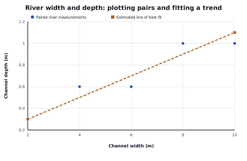
Suppose these river measurements were collected. The separate points show a positive relationship; the fitted line summarises the trend rather than connecting the observations.
Data for River width and depth: plotting pairs and fitting a trend
| Series | Channel width (m) | Channel depth (m) |
|---|---|---|
| Paired river measurements | 2 | 0.3 |
| Paired river measurements | 4 | 0.6 |
| Paired river measurements | 6 | 0.6 |
| Paired river measurements | 8 | 1 |
| Paired river measurements | 10 | 1 |
| Estimated line of best fit | 2 | 0.3 |
| Estimated line of best fit | 10 | 1.1 |
Read the pattern from left to right. Here, greater widths are generally associated with greater depths, so there is a positive correlation. A downward pattern would show a negative correlation: as one variable increases, the other generally decreases. If the points have no clear upward or downward pattern, there is no clear correlation.
The closer the points lie to a clear trend, the stronger the relationship. Widely scattered points indicate a weaker relationship. A useful geographical description names both variables and recognises that a trend need not apply perfectly to every observation: ‘Wider river channels tend to be deeper.’
A line of best fit summarises the overall pattern rather than linking the points. For a roughly straight relationship, position a ruler through the middle of the point cloud and draw a single straight line across the data range. Aim for roughly balanced numbers of points above and below it along its length, while keeping the line close to the overall pattern.
A point far from the main pattern is an outlier. Do not let one isolated outlier pull the line away from the main group. A trend line can be curved where the pattern clearly curves; a straight line should not be forced onto every relationship. With no clear correlation, a fitted line would not provide useful predictions.
The river graph includes one reasonable estimated line. Another carefully drawn line could give slightly different estimates because fitting it by eye is an approximation.
To predict depth for a width of 7 m, move vertically from 7 m on the horizontal axis to the fitted line, then horizontally to the depth axis. The estimate is about 0.8 m. This is interpolation because 7 m lies within the recorded width range of 2–10 m.
The prediction describes a likely value, not a guaranteed depth at every 7 m-wide site. Points scatter around the line, and other river characteristics may affect depth. Correlation alone also does not prove that one variable causes the other. Stronger, clearer patterns generally support more confident predictions than weak patterns.
A line graph connects values in an ordered sequence, often through time. Suppose a park recorded 100,000 visitors in year 1, 140,000 in year 3 and 180,000 in year 5.
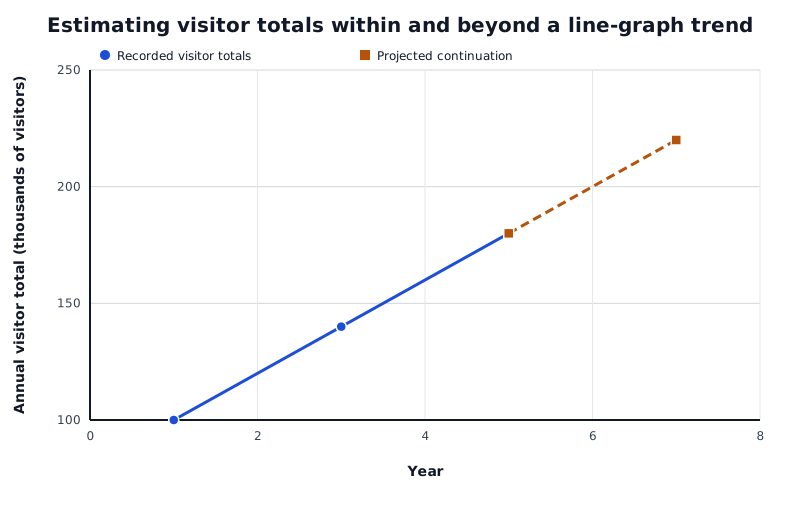
Suppose a park recorded these visitor totals. Read between the recorded years to interpolate; the projected extension assumes the same upward trend continues.
Data for Estimating visitor totals within and beyond a line-graph trend
| Series | Year | Annual visitor total (thousands of visitors) |
|---|---|---|
| Recorded visitor totals | 1 | 100 |
| Recorded visitor totals | 3 | 140 |
| Recorded visitor totals | 5 | 180 |
| Projected continuation | 5 | 180 |
| Projected continuation | 7 | 220 |
To interpolate the visitor total for year 4, move up from year 4 to the line between years 3 and 5, then across to the vertical axis. The reading is 160 thousand, or 160,000 visitors. This estimate assumes that the change between the two recorded years follows the straight connecting line.
To extrapolate, extend the established trend beyond the last recorded value. Here, the total rises by 40,000 visitors every two years. Continuing that trend to year 7 gives 220,000 visitors.
Extrapolation is less secure because there are no recorded values in that extended range. It assumes the trend continues, although visitor numbers could level off or fall. State the prediction conditionally: ‘If the recent trend continues, the park would receive about 220,000 visitors in year 7.’
Describe a relationship using both variable names: for example, ‘As river width increases, river depth generally increases.’
Do not join the individual points on a scatter plot. Draw a separate estimated line of best fit through the overall pattern.
A line of best fit does not have to pass through the origin or any particular data point.
Read predictions from the trend line, not from the nearest individual point, and include the units.
When explaining uncertainty in an extrapolation, state that it lies beyond the recorded data range and assumes the trend continues.
It can see this note and what your specification asks for.
Answers are free with an account.
1 free note left this week
Get more free notesYour answer sets when this note comes back for review, or marks it complete.
Was this note helpful?
Log in to tell us whether it helped, or to report a problem.
Last updated
Bivariate data
Paired information about two variables for each observation, such as river width and depth at each sampling site.
Scatter plot
A graph in which each point represents a pair of numerical values, used to investigate the relationship between two variables.
Correlation
A pattern of association between two variables. It is positive when they tend to increase together and negative when one tends to decrease as the other increases.
Line of best fit
A line drawn through the overall pattern of a scatter plot to summarise the relationship and estimate values.
Outlier
A data point that lies noticeably away from the general pattern of the other points.
Interpolation
Estimating a value within the range covered by the recorded data.
Extrapolation
Estimating a value beyond the range covered by the recorded data by extending its trend.
Put your knowledge into practice — try past paper questions for Geography B
Bivariate data
Paired information about two variables for each observation, such as river width and depth at each sampling site.
Scatter plot
A graph in which each point represents a pair of numerical values, used to investigate the relationship between two variables.
Correlation
A pattern of association between two variables. It is positive when they tend to increase together and negative when one tends to decrease as the other increases.
Line of best fit
A line drawn through the overall pattern of a scatter plot to summarise the relationship and estimate values.
Outlier
A data point that lies noticeably away from the general pattern of the other points.
Interpolation
Estimating a value within the range covered by the recorded data.
Extrapolation
Estimating a value beyond the range covered by the recorded data by extending its trend.