

Loading…
Loading…
Loading…
Eduqas GCSE Geography A · C111
Eduqas C111 · Graphical Skills Check the specification (PDF) (opens in a new tab)
A graph turns a table of measurements into a picture that helps you compare places, recognise changes or investigate relationships. Choosing a graph starts with asking what the data represents and what you want to show.
Counts, such as numbers of visitors, are discrete data: separate values. Measurements such as temperature and depth are continuous data: values anywhere within a range. Categories such as transport types are separate groups, even when the number recorded for each group is numerical.
Use a bar chart to compare categories, a line chart to show an ordered change, and a pie chart to show parts of one total. Other graphs have more specialised jobs: a histogram shows grouped measurements, a dispersion graph shows their spread, and a scatter graph investigates a relationship between two variables.
First identify the variables, units, smallest and largest values. Choose a scale that fits the data and uses the available space effectively. If visitor counts range from 0 to 46, a vertical scale from 0 to 50 in intervals of 5 would be convenient. Each equal distance on that axis must represent the same numerical increase.
Give the graph a descriptive title. Label axes with both the variable and unit, such as ‘Distance downstream (km)’. Add a key when colours, symbols or several datasets need distinguishing. Bar charts normally start their value scale at zero because bar length represents quantity. If an axis is shortened, make the break clear: changing a scale can make a difference appear much larger or smaller.
Construction is complete when all values are plotted, labels and keys are present, and the finished graph has been checked against the original table.
For a bar chart, place categories along one axis and values along the other. Draw bars of equal width with equal gaps between them. Suppose pedestrian counts at three sites are 12, 28 and 20 people during the same observation period. On a scale marked every 5 people, their bars reach 12, 28 and 20. Site B has the largest count, exceeding Site A by 16 people. The graph establishes that difference, but does not explain its cause.
For a line chart, put the ordered variable, often time or distance, on the horizontal axis. Plot each pair of values accurately and join consecutive points. Position points according to their numerical values: observations at 0, 2 and 5 km must not be equally spaced along a distance axis.
A line helps reveal increases, decreases and turning points. Its steepness shows how rapidly the vertical variable changes relative to the horizontal variable. A flat section shows little or no change. Joining points suggests change between observations; it does not mean every intermediate value was measured.
A climate chart combines precipitation bars and a temperature line for the twelve months. The values are usually long-term monthly averages. Months run from January to December along the horizontal axis; precipitation has a scale in millimetres and temperature has a separate scale in degrees Celsius.
To construct one, draw the precipitation bars against their scale, then plot and join the temperature points against the temperature scale. Keeping the two scales separate matters because millimetres and degrees Celsius are different quantities.
Read a climate chart by identifying the hottest and coldest months, the wettest and driest months, and seasonal patterns. The annual temperature range is the highest monthly mean minus the lowest. Total annual precipitation is the sum of the twelve monthly precipitation values. Monthly averages conceal daily extremes and variations between years.
A hydrograph shows river discharge over time. Discharge is the volume of water passing a point each second, measured in cubic metres per second, . A storm hydrograph combines rainfall bars, read in millimetres, with a discharge line, read from its own scale.
Plot rainfall for each stated time interval and plot discharge at the stated times. The rising limb is the increase in discharge; peak discharge is its highest value; the falling limb shows discharge decreasing afterwards. Lag time is the time between peak rainfall and peak discharge. Use the centre of the highest rainfall bar to locate its time.
Suppose peak rainfall is centred on 02:00 and peak discharge occurs at 05:00. The lag time is three hours. This delay reflects the time water takes to reach the river. A steep rising limb indicates a rapid response, while a gentler one indicates a slower response. The graph alone cannot establish which catchment characteristic caused that response.
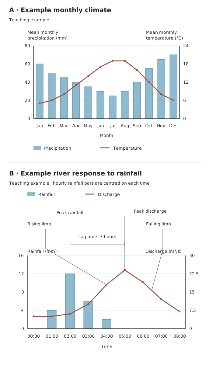
Two variables can share a time axis, but each must be read from its own value scale. The storm hydrograph has a three-hour lag time.
A pie chart divides a circle into sectors representing parts of one whole. Calculate the total first, then convert each category into an angle:
Suppose a transport survey records 20 walkers, 30 bus users and 50 car users: 100 people altogether. The sectors are , and . Draw a circle, mark successive angles with a protractor, and label or colour the sectors with a key. Check that the angles total . The chart shows that half the sample travels by car; without the total, percentages alone would not tell you how many people that represents.
Proportional circles compare quantities through circle area. Select a reference circle and use the same area scale for every value. If 100 visitors are represented by a circle of radius 1 cm, 400 visitors need four times its area, so the radius is 2 cm. This follows from : doubling the radius quadruples the area.
More generally:
Label the circles or provide a size key. Proportional circles show differences in total quantity; pie sectors show the composition of a total. These are different teaching jobs even when the two methods are combined.
A pictogram repeats a symbol, with each symbol representing a fixed quantity. Choose a simple symbol and state its value in a key. Suppose one visitor symbol represents 10 visitors. Counts of 20, 35 and 50 visitors require two, three-and-a-half and five symbols. Keep whole symbols the same size and use a clearly recognisable half-symbol where needed. Compare the quantities after applying the key, rather than assuming one symbol always means one item.
A histogram shows how often measurements fall within class intervals. For this course, use equal class intervals. Place the intervals on a continuous horizontal scale and frequency on the vertical axis. Draw touching bars: the intervals are adjoining ranges, not separate categories.
Suppose ten river-depth measurements are grouped as follows:
| Depth interval | Frequency |
|---|---|
| 0 cm up to, but not including, 10 cm | 2 |
| 10 cm up to, but not including, 20 cm | 5 |
| 20 cm up to, but not including, 30 cm | 3 |
Draw three bars covering 0–10, 10–20 and 20–30 cm, with heights 2, 5 and 3. A depth of exactly 10 cm belongs in the second interval, so it is not counted twice. The most frequent interval is 10–20 cm. Grouping makes the distribution clearer, but you cannot recover each individual depth from the histogram.
Star and radial graphs use axes radiating from a centre. They are useful for displaying several related measurements, such as environmental-quality scores for cleanliness, noise, vegetation and building condition.
Label one spoke for each component and mark a consistent scale. For a star-style graph, plot the score on each spoke and join neighbouring points to create a closed shape. A radial display can also use bars or separate lines extending along the spokes. Read the labelled scales rather than relying only on the overall shape.
Suppose each environmental component is scored from 0 to 5, with larger values always meaning better quality. Scores of 4 for cleanliness, 2 for quietness, 5 for vegetation and 3 for building condition show that vegetation is the strongest component and quietness the weakest. A second site's outline can be added using the same axes, order and scale. Changing the order of the spokes changes the shape, so comparisons require a consistent layout.
A kite diagram shows where something occurs along a transect and how abundant it is. Distance along the transect forms the horizontal axis. Each species has its own horizontal centre line, and the kite extends equally above and below that line. Its width represents abundance according to a stated scale.
Suppose grass counts at 0, 10 and 20 m are 2, 6 and 0 plants. Choose a total kite width of 1 mm per plant. At those positions, mark 1, 3 and 0 mm above the centre line and the same distances below it. Join the upper points and lower points, then shade the kite. It is widest at 10 m, where grass is most abundant, and narrows to zero at 20 m.
Separate centre lines allow several species to be compared at the same distances. Use the same abundance scale throughout. The diagram reveals distribution and abundance along the sampled line, not across the whole habitat.
A triangular graph represents three components of one total, such as percentages employed in primary, secondary and tertiary activities. Each side carries a scale from 0% to 100%. The three percentages for every observation must total 100%.
Follow each printed scale carefully: the values may increase in different directions. A line of constant percentage for one component runs parallel to the side opposite that component's 100% corner. Find the first percentage on its scale and trace the corresponding line into the triangle. Repeat for the second component. Their intersection is the point; check it against the third percentage.
Suppose employment is 20% primary, 30% secondary and 50% tertiary. The three percentage lines meet at one point. A point nearer the primary corner represents a larger primary share. Several points close together have similar compositions. The graph compares proportions, not total numbers employed.
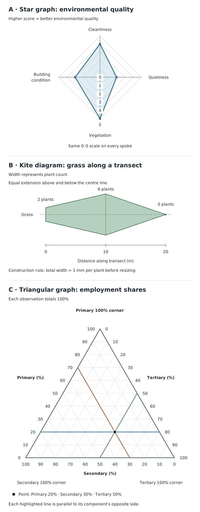
Spoke distance shows a component score, kite width shows abundance, and a triangular point shows three shares of one total.
A dispersion graph displays the individual values in each dataset so that their spread can be compared. Put the sites or groups along the horizontal axis and the measured variable on a common vertical scale. Plot each observation as a separate point above its group. Keep repeated values visible by placing their dots close together at the same height.
Suppose noise readings at Site A are 40, 42 and 44 dB, and at Site B are 30, 42 and 54 dB. Both sets have a mean of 42 dB, but their ranges are 4 dB and 24 dB. Site B's readings are much more variable. Showing only the means would hide that difference.
A scatter graph instead plots paired measurements to investigate a relationship. For example, each river site could supply one pair: channel width on the horizontal axis and channel depth on the vertical axis. Plot one point for each pair without joining the points in observation order.
An upward pattern suggests positive correlation; a downward pattern suggests negative correlation. A scattered cloud without a clear direction suggests little or no correlation. If appropriate, draw a line of best fit through the middle of the pattern, with roughly balanced points on either side. Identify anomalies separately. Even a strong relationship does not, by itself, prove cause and effect.
Begin by checking the title, dates, variables, units, scales and key. Extract values by tracing from a bar, point, line or sector to the relevant scale. Then describe the overall pattern before adding detail: an increase, a seasonal cycle, a concentration of values, a contrast between groups or a correlation.
Support your description with values, units and locations or times. ‘Site B has more pedestrians’ is less informative than ‘Site B records 28 pedestrians, compared with 12 at Site A’. Include an important exception if one exists.
Finally, distinguish description from explanation. A graph can show that values differ or move together, but explaining why usually needs geographical knowledge or additional evidence. Consider what the display conceals: grouped values hide individual measurements, percentages hide total size, and averages hide variation.
| Purpose | Suitable graph |
|---|---|
| Compare separate categories | Bar chart |
| Show change over time or distance | Line chart |
| Monthly precipitation and temperature | Climate chart: bars and line |
| River discharge over time | Hydrograph; storm hydrograph adds rainfall bars |
Label axes with the variable and unit, use evenly spaced numerical intervals, and include a clear title and any necessary key.
Keep gaps between bars for separate categories; use touching bars for a histogram with equal class intervals.
On a climate chart or hydrograph, read each variable from its own labelled scale.
Make proportional-circle areas proportional to the values, not their radii or diameters.
For triangular graphs, check that the three percentages total 100% and follow the direction of each printed scale.
Support descriptions of patterns with figures and units. Mention important exceptions rather than claiming every value follows the pattern.
Do not join scatter-graph points in sequence. Correlation alone does not prove that one variable causes another.
It can see this note and what your specification asks for.
Answers are free with an account.
1 free note left this week
Get more free notesYour answer sets when this note comes back for review, or marks it complete.
Was this note helpful?
Log in to tell us whether it helped, or to report a problem.
Last updated
Discrete data
Numerical data consisting of separate, countable values, such as the number of vehicles passing a site.
Continuous data
Numerical data that can take any value within a range, such as temperature or river depth.
Frequency
The number of observations belonging to a particular value, category or class interval.
Class interval
A range used to group numerical observations, such as depths from 0 cm up to, but not including, 10 cm.
Hydrograph
A graph showing how river discharge changes over time; a storm hydrograph also displays rainfall.
Discharge
The volume of water passing a point in a river each second, usually measured in .
Lag time
The time between peak rainfall and peak river discharge on a storm hydrograph.
Histogram
A graph of grouped continuous data using touching bars. With equal class intervals, bar height represents frequency.
Radial graph
A graph with several axes radiating from a central point, used to compare related components of data.
Transect
A line along which observations or measurements are collected at different positions.
Correlation
A relationship between two variables: positive when they tend to increase together, or negative when one tends to decrease as the other increases.
Anomaly
A value or observation that differs noticeably from the general pattern of a dataset.
Put your knowledge into practice — try past paper questions for Geography A
Discrete data
Numerical data consisting of separate, countable values, such as the number of vehicles passing a site.
Continuous data
Numerical data that can take any value within a range, such as temperature or river depth.
Frequency
The number of observations belonging to a particular value, category or class interval.
Class interval
A range used to group numerical observations, such as depths from 0 cm up to, but not including, 10 cm.
Hydrograph
A graph showing how river discharge changes over time; a storm hydrograph also displays rainfall.
Discharge
The volume of water passing a point in a river each second, usually measured in .
Lag time
The time between peak rainfall and peak river discharge on a storm hydrograph.
Histogram
A graph of grouped continuous data using touching bars. With equal class intervals, bar height represents frequency.
Radial graph
A graph with several axes radiating from a central point, used to compare related components of data.
Transect
A line along which observations or measurements are collected at different positions.
Correlation
A relationship between two variables: positive when they tend to increase together, or negative when one tends to decrease as the other increases.
Anomaly
A value or observation that differs noticeably from the general pattern of a dataset.
| Show parts of one total | Pie chart |
| Compare quantities by area | Proportional circles |
| Show counts using repeated symbols | Pictogram |
| Show grouped continuous measurements | Histogram with equal class intervals |
| Compare several components | Star or radial graph |
| Show abundance along a transect | Kite diagram |
| Show three percentages totalling 100% | Triangular graph |
| Compare spread within datasets | Dispersion graph |
| Investigate two paired variables | Scatter graph |
Check title, units, scales and key → identify the overall pattern → support it with figures → note exceptions.
Distinguish positive, negative and little or no correlation. Patterns do not prove causes. Check whether totals, variation or individual values are hidden by the chosen display.