

Loading…
Loading…
Loading…
OCR GCSE Geography A · J383
OCR J383 · Types of Graphs and Charts Check the specification (PDF) (opens in a new tab)
Different graphs reveal different things about geographical data. A bar graph compares separate sites or categories. A histogram shows how continuous measurements are distributed across size ranges. A line graph shows change along a continuous scale, while a scatter graph investigates a relationship between two numerical variables.
The choice depends on how the data are organised, not simply whether they contain numbers. River cross-sectional area is a continuous measurement, but a bar graph can compare its value at five separate sampling sites. Pebble lengths grouped into consecutive size intervals need a histogram instead.
An ordinary bar graph represents each category with a separate bar. In a vertical bar graph, categories go along the horizontal axis and bar heights show their values. Use equal-width bars and equal gaps: the gaps show that the categories are separate.
A horizontal bar graph works in the same way, but categories run down the vertical axis and bar lengths are read against a horizontal numerical scale. This can make long category names easier to read. To construct either version, label the categories, choose a numerical scale starting at zero, and draw each bar to the correct value.
For example, mean river cross-sectional area is the average area of a slice across a river channel, measured in square metres. At the five River Holford sites in Somerset, the values rise from about 0.5 m² at Site 1 to 2.3 m² at Site 5. The bars therefore show an overall increase across the numbered sites. Site 5 has the largest value; the increase is not the same between every pair of sites.
A divided bar graph shows the components making up a total. Each bar is split into labelled or keyed segments and can be drawn horizontally or vertically. Read a segment's size by subtracting its starting position from its ending position, rather than treating its endpoint as its value.
Suppose a land-use survey records 40 premises: 20 shops, 10 offices and 10 homes. A count-based divided bar would have a total length of 40, with segment boundaries at 20, 30 and 40. The office segment is 10 premises long, not 30. To construct it horizontally, use a horizontal scale labelled 'Number of premises', draw the whole bar from 0 to 40, then divide it at 20 and 30. Shade each land-use category differently and provide a key. If comparing several survey areas, keep the category order and shading consistent across the bars.
A percentage divided bar makes every whole bar represent 100%, allowing composition to be compared when totals differ:
In this example, shops occupy 50% of the bar, offices 25% and homes 25%. Use a scale from 0 to 100%, with boundaries at 50%, 75% and 100%. A percentage bar shows proportions, but its equal total length does not mean that different surveys counted equal numbers of premises.
Pebble length is continuous: a pebble could measure 3 cm, 3.2 cm or a value between them. A histogram groups these measurements into class intervals and shows how many observations fall in each interval.
For the equal-class-interval histograms studied here, put the measurement and its units on the horizontal axis and frequency on the vertical axis. Draw bars across the full interval widths, with no gaps between neighbouring intervals. Their touching edges represent the continuous measurement scale. Because all intervals have equal widths, taller bars directly indicate more observations.
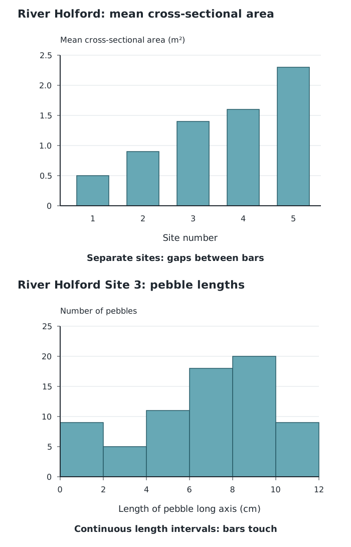
Separate river sites are compared with a bar graph; continuous pebble lengths are grouped into equal intervals in a histogram.
The River Holford pebble sample from Site 3 uses intervals 2 cm wide. The 8–10 cm interval contains 20 pebbles, whereas the 2–4 cm interval contains five. This makes 8–10 cm the most frequent size class; it does not mean that every pebble in that class measured exactly 8 cm or 10 cm.
To construct a similar histogram, group measurements into non-overlapping intervals, count the observations in each one, and draw touching bars to those frequencies. Set a boundary rule so that a measurement exactly on an interval boundary is counted only once—for example, 2 cm up to but not including 4 cm.
A line graph is useful when the horizontal axis represents a continuous sequence, such as time or distance. Plot each pair of values and join neighbouring points in order. The line makes increases, decreases and periods of little change easier to see.
The River Eea in Cumbria was sampled at six distances from its source. These distances are unevenly spaced: 0.5, 0.8, 1.3, 1.7, 2.1 and 3 km. Their positions on the graph must preserve those distances rather than giving every sampling site the same gap.
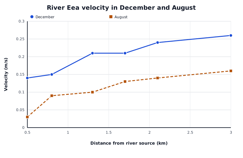
December and August velocities at six sampled distances along the River Eea. Unequal distances between sites are retained on the horizontal scale.
Data for River Eea velocity in December and August
| Series | Distance from river source (km) | Velocity (m/s) |
|---|---|---|
| December | 0.5 | 0.14 |
| December | 0.8 | 0.15 |
| December | 1.3 | 0.21 |
| December | 1.7 | 0.21 |
| December | 2.1 | 0.24 |
| December | 3 | 0.26 |
| August | 0.5 | 0.03 |
| August | 0.8 | 0.09 |
| August | 1.3 | 0.1 |
| August | 1.7 | 0.13 |
| August | 2.1 | 0.14 |
| August | 3 | 0.16 |
December velocity increases overall from 0.14 m/s at 0.5 km to 0.26 m/s at 3 km, although it stays at 0.21 m/s between 1.3 and 1.7 km. August also shows an overall increase, but its values are lower than December's at every sampled distance.
Multiple lines allow comparisons at the same x-value. At 3 km, December velocity is 0.26 m/s and August velocity is 0.16 m/s: a difference of 0.10 m/s. Use a key so that each line can be identified. The connecting lines help show the pattern between sampled points; they do not establish that every intermediate location was measured.
A scatter graph plots two numerical measurements for each observation. For example, one observation might pair distance from an urban centre with noise level at that location. Put one variable on each axis and plot a point where its two values meet. Do not join the observations in sequence.
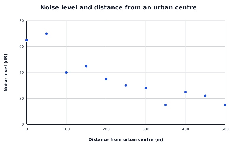
The overall downward pattern shows negative correlation between distance from the urban centre and noise level.
Data for Noise level and distance from an urban centre
| Series | Distance from urban centre (m) | Noise level (dB) |
|---|---|---|
| Noise level | 0 | 65 |
| Noise level | 50 | 70 |
| Noise level | 100 | 40 |
| Noise level | 150 | 45 |
| Noise level | 200 | 35 |
| Noise level | 250 | 30 |
| Noise level | 300 | 28 |
| Noise level | 350 | 15 |
| Noise level | 400 | 25 |
| Noise level | 450 | 22 |
| Noise level | 500 | 15 |
Here, noise levels generally decrease as distance from the urban centre increases. This is negative correlation. For instance, the plotted noise level is 70 dB at 50 m and 15 dB at 500 m. Not every point follows a perfectly smooth decrease, so describe the overall relationship rather than claiming that all observations behave identically.
A positive correlation slopes upwards overall: as one variable increases, the other tends to increase. With no clear correlation, the points show no consistent upward or downward pattern. A narrow band of points indicates a stronger relationship than a widely scattered pattern.
To draw a straight line of best fit, look at the whole cloud of points and place the line through its centre, close to as many points as possible, with roughly balanced numbers above and below it. It need not pass through every point or the origin. Points far from the overall pattern deserve investigation, but should not automatically be deleted.
The line can help estimate a value within the observed range: move from a chosen x-value to the line, then across to the y-axis. Such estimates are approximate. Extending the relationship beyond the observed range is less secure, and correlation by itself does not establish a cause.
Give each axis a label and units where relevant. For horizontal bars, the numerical scale is on the horizontal axis.
Keep equal gaps between ordinary bars, but make histogram bars touch. This lesson requires histograms with equal class intervals.
On a divided bar, distinguish the size of each segment from the cumulative position of its endpoint. Include a key.
Space line-graph points according to their numerical x-values, not equally just because they appear in successive table rows.
Do not join scatter-graph points dot to dot. Draw a straight line of best fit through the overall pattern, aiming for roughly balanced numbers of points above and below it.
Support descriptions with values and units. A correlation alone does not prove that one variable causes another.
It can see this note and what your specification asks for.
Answers are free with an account.
1 free note left this week
Get more free notesYour answer sets when this note comes back for review, or marks it complete.
Was this note helpful?
Log in to tell us whether it helped, or to report a problem.
Last updated
Discrete data
Data consisting of separate categories or distinct values, rather than every possible value along a continuous scale.
Continuous data
Measurements that can take any value within a range, such as distance or pebble length.
Bar graph
A graph using separate bars to compare values for different categories or discrete observations.
Divided bar graph
A bar split into segments to show how different components contribute to a total.
Histogram
A graph showing the frequency distribution of continuous data grouped into intervals, with adjacent bars touching.
Class interval
A range of values used to group measurements, such as pebble lengths from 2 cm up to 4 cm.
Frequency
The number of observations in a category or class interval.
Line graph
A graph in which plotted points are joined in order to show change along a continuous scale, such as time or distance.
Scatter graph
A graph plotting paired values of two numerical variables to investigate their relationship.
Correlation
The direction and strength of a relationship between two variables.
Line of best fit
A line drawn through the overall pattern of points on a scatter graph to summarise their relationship.
Put your knowledge into practice — try past paper questions for Geography A
Discrete data
Data consisting of separate categories or distinct values, rather than every possible value along a continuous scale.
Continuous data
Measurements that can take any value within a range, such as distance or pebble length.
Bar graph
A graph using separate bars to compare values for different categories or discrete observations.
Divided bar graph
A bar split into segments to show how different components contribute to a total.
Histogram
A graph showing the frequency distribution of continuous data grouped into intervals, with adjacent bars touching.
Class interval
A range of values used to group measurements, such as pebble lengths from 2 cm up to 4 cm.
Frequency
The number of observations in a category or class interval.
Line graph
A graph in which plotted points are joined in order to show change along a continuous scale, such as time or distance.
Scatter graph
A graph plotting paired values of two numerical variables to investigate their relationship.
Correlation
The direction and strength of a relationship between two variables.
Line of best fit
A line drawn through the overall pattern of points on a scatter graph to summarise their relationship.