

Loading…
Loading…
Loading…
OCR GCSE Geography A · J383
OCR J383 · Types of Graphs and Charts Check the specification (PDF) (opens in a new tab)
Choosing a graph depends on what you want to find out. A dispersion graph reveals how much observations vary. A pie chart shows how a total is divided. A climate graph brings temperature and precipitation together. Proportional symbols show quantities at locations, while pictograms make category totals easy to compare.
Before reading any of them, check the title, labels, units and key. These establish what the data represents and how to turn a mark, sector or symbol into a value.
An average can hide considerable variation. A dispersion graph plots each observation separately, usually on a vertical numerical scale, with different datasets arranged side by side. Unlike a scatter graph, its purpose is not to show a relationship between two numerical variables: it shows the spread within and between datasets.
Suppose wind speeds are recorded five times at each of two sites. Site A has speeds of 2, 3, 4, 5 and 8 m/s; Site B has speeds of 3, 3.5, 4, 4.5 and 5 m/s.
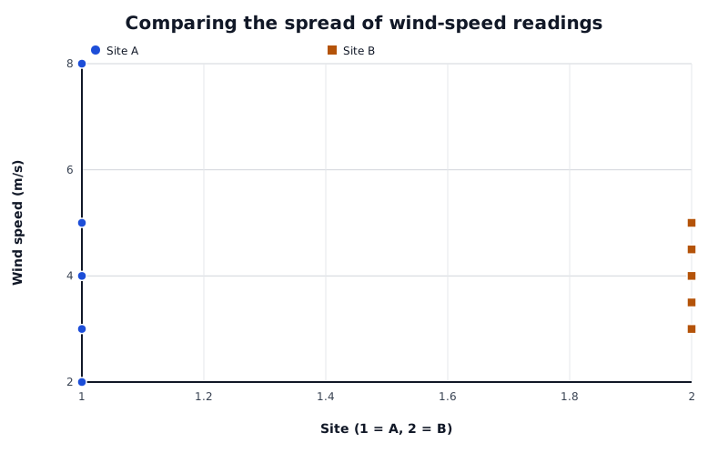
Both sites have a median wind speed of 4 m/s, but Site A has the wider range.
Data for Comparing the spread of wind-speed readings
| Series | Site (1 = A, 2 = B) | Wind speed (m/s) |
|---|---|---|
| Site A | 1 | 2 |
| Site A | 1 | 3 |
| Site A | 1 | 4 |
| Site A | 1 | 5 |
| Site A | 1 | 8 |
| Site B | 2 | 3 |
| Site B | 2 | 3.5 |
| Site B | 2 | 4 |
| Site B | 2 | 4.5 |
| Site B | 2 | 5 |
Read the lowest and highest points first. Site A has a range of , whereas Site B has a range of . Both have a middle value, or median, of 4 m/s, but Site A's readings are much more spread out. This shows why a typical value alone does not fully describe a dataset.
Look also for clusters and isolated points. Site A's 8 m/s reading stands apart from its other readings, making it a possible outlier. An unusual value is not automatically a mistake: it may represent a genuine gust. A tighter cluster indicates more consistent readings, but does not by itself prove that measurements are accurate.
To plot a dispersion graph, choose a suitable numerical scale, label it with units and mark each observation in its dataset's column. If readings repeat, show their frequency clearly rather than losing several observations beneath one dot. Do not join the points.
A pie chart represents a whole as a circle. Each category occupies a sector, and all the sectors together represent 100%, or . Read the key to identify each category, then use the percentage labels or sector angles to establish its share.
For example, an energy mix can contain coal at 38%, oil at 22%, gas at 15%, nuclear at 5% and renewables at 20%. Coal is the largest individual category, but it does not provide a majority. Coal, oil and gas together account for 75% of the total.
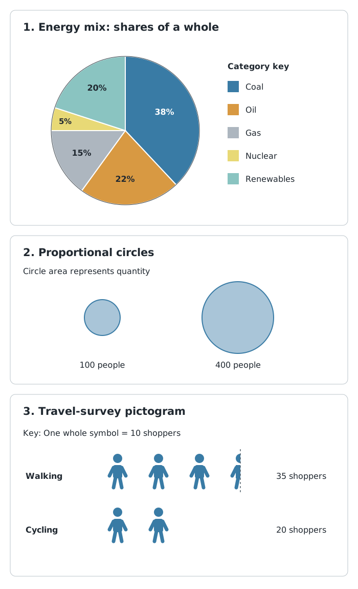
Sectors show shares, circle areas show quantities, and repeated symbols show counts.
To construct a pie chart from counts, first find the total. Convert each count into a sector angle using:
For percentage data, multiply each percentage by 3.6. A 20% share therefore occupies . Draw the sectors with a protractor, and add a title and clear labels or a key.
Pie charts make broad proportions easy to see, but similar-sized or very small sectors are harder to compare. They do not show the total amount unless that information is supplied separately. Two places could both obtain 20% of their energy from renewables while using very different amounts of energy overall.
Climate describes long-term weather patterns. A climate graph usually uses long-term monthly averages, commonly calculated over 30 years, rather than the weather during one particular year.
The horizontal axis runs from January to December. Bars show monthly precipitation in millimetres, and a line shows mean monthly temperature in degrees Celsius. These use separate vertical scales: check which side belongs to each variable rather than assuming a fixed layout.
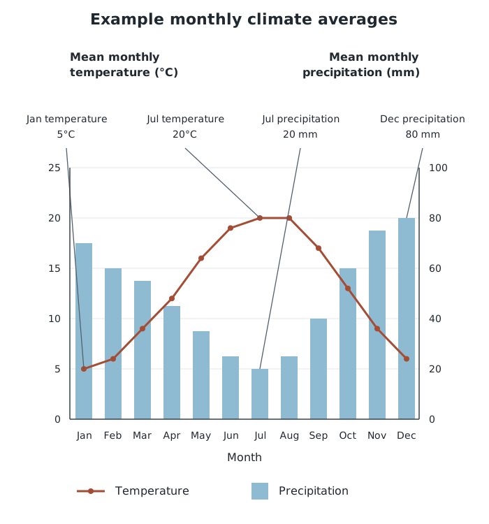
Read each variable from its own scale: this example has warmer, drier middle months and cooler, wetter end months.
Suppose a place has the monthly averages shown in the graph. Follow the temperature line to identify the warmest and coldest months. July is warmest at 20°C and January is coldest at 5°C, so the annual temperature range is .
Next, read the precipitation bars. December is wettest at 80 mm and July is driest at 20 mm. Together, the line and bars show a pattern of warmer, drier conditions in the middle of the year and cooler, wetter conditions towards its beginning and end.
Annual precipitation is found by adding all twelve monthly precipitation values. Do not add monthly temperatures to obtain annual temperature: an annual mean is an average, not a total.
When describing a climate graph, cover both variables and their seasonal patterns, using figures as evidence. When comparing places, compare temperature levels, annual temperature range, precipitation totals and the distribution of precipitation through the year. Monthly averages hide daily extremes and differences between individual years, so the graph cannot tell you whether a particular day experienced a storm or heatwave.
Proportional symbols connect quantity with location. They can show features such as population, electricity generation or traffic flows. Each symbol is placed at the location it represents, and a key links symbol sizes to values.
For circles, the area—not the diameter—is proportional to the quantity. In the example above, a circle representing 400 people has four times the area of one representing 100 people, but only twice its diameter.
Read a proportional-symbol map by checking the variable and units, comparing symbols with the key, and then looking for concentrations of larger or smaller values. Explain the spatial pattern using place names or directions supported by the actual map. The simple circle comparison here demonstrates size scaling; it does not locate a real population or establish a geographical pattern.
These maps make differences between places easy to recognise, but exact values can be difficult to estimate. Large symbols may overlap and obscure locations. They show the amount at each marked location, not how evenly that amount is distributed around it.
A pictogram uses repeated symbols to show category totals. Its key is essential: one picture may represent one person, ten people or another stated amount. Partial symbols represent the corresponding fraction of that amount.
Suppose a travel survey uses one symbol for 10 shoppers. Three whole symbols and a half-symbol in the walking row represent 35 shoppers; two whole symbols in the cycling row represent 20. Walking therefore accounts for 15 more shoppers than cycling.
To read a pictogram, select the relevant row, count the whole and partial symbols, and multiply by the value in the key. A picture used as a row label is not part of the data count. To construct one, choose a manageable value per symbol, use equally sized symbols, align the rows and include a title, category labels and key.
Pictograms communicate simple totals quickly, especially for discrete counts such as numbers of shoppers. However, awkward fractions and large numbers of symbols can make precise comparisons difficult. They are useful for clear visual comparisons, not for showing every detail of a complex dataset.
Support a description of a pattern with figures and units, then mention any important exception.
On a climate graph, read temperature and precipitation from their own axes: the scales are different.
A change from 20% to 30% is 10 percentage points, not a 10% increase.
Use the key before counting pictogram symbols, and include fractions of symbols.
For proportional circles, compare area rather than diameter. A circle with twice the diameter has four times the area.
The largest category is not necessarily a majority: a majority means more than half.
It can see this note and what your specification asks for.
Answers are free with an account.
1 free note left this week
Get more free notesYour answer sets when this note comes back for review, or marks it complete.
Was this note helpful?
Log in to tell us whether it helped, or to report a problem.
Last updated
Dispersion graph
A graph showing individual values in a dataset so that their spread, clusters and unusual values can be compared.
Range
The difference between the highest and lowest values in a dataset: .
Outlier
A value that lies noticeably apart from the main group of values.
Pie chart
A circle divided into sectors whose sizes show the proportions of categories within a whole.
Climate graph
A graph combining monthly precipitation bars and a mean monthly temperature line to show the climate of a place.
Precipitation
Water reaching the ground from the atmosphere, including rain, snow, sleet and hail.
Proportional symbol
A symbol whose size represents the quantity at a location; for proportional circles, area is proportional to the value.
Pictogram
A chart using repeated pictures or symbols to represent quantities, with a key giving the value of each symbol.
Put your knowledge into practice — try past paper questions for Geography A
Dispersion graph
A graph showing individual values in a dataset so that their spread, clusters and unusual values can be compared.
Range
The difference between the highest and lowest values in a dataset: .
Outlier
A value that lies noticeably apart from the main group of values.
Pie chart
A circle divided into sectors whose sizes show the proportions of categories within a whole.
Climate graph
A graph combining monthly precipitation bars and a mean monthly temperature line to show the climate of a place.
Precipitation
Water reaching the ground from the atmosphere, including rain, snow, sleet and hail.
Proportional symbol
A symbol whose size represents the quantity at a location; for proportional circles, area is proportional to the value.
Pictogram
A chart using repeated pictures or symbols to represent quantities, with a key giving the value of each symbol.