

Loading…
Loading…
Loading…
AQA GCSE Statistics · 8382
AQA 8382 · 3.3.3 Constructing and Interpreting Charts and Graphs Check the specification (PDF) (opens in a new tab)
A frequency tells you how many observations have a particular value or fall within a particular group. A distribution shows how those observations are spread across the possible values. When interpreting a graph, first establish what is being measured, its units, and what the vertical scale represents.
Two useful questions are: where do the values tend to lie, and how spread out are they? A group can have a lower typical value but a greater spread, so neither question answers the other.
A bar line chart, also called a vertical line graph, represents discrete numerical data with vertical lines rather than rectangular bars. Each line stands above a possible data value, and its height gives the frequency. The lines are not joined together.
Suppose 14 pupils report how many books they read in a month:
| Books read | Frequency |
|---|---|
| 0 | 3 |
| 1 | 5 |
| 2 | 4 |
| 3 | 2 |
The line above 1 reaches a frequency of 5, so 1 book is the mode: it is the most common value. The line heights total 14, the number of pupils. To find how many read at least 2 books, combine the frequencies for 2 and 3: there are 6 pupils.
To compare two bar line charts, look for differences in their most common values and in the extent of the values. Use matching scales, and check the group sizes: a taller line may simply come from a larger group.
Continuous measurements, such as time or mass, can take values between whole numbers. They are often collected into class intervals. For example, includes times from 10 minutes up to, but not including, 20 minutes.
A histogram places each class interval along the horizontal axis. Its rectangles touch because adjacent intervals cover adjoining parts of a continuous scale. For equal-width classes, a vertical frequency scale can be used, so the height of each rectangle gives its frequency.
A frequency polygon shows the same grouped frequencies in a different way. Each frequency is plotted above the midpoint of its class, and consecutive points are joined with straight lines. The midpoint is halfway between the class boundaries.
Suppose the journey times of 40 commuters are grouped as follows:
| Journey time, minutes | Frequency | Class midpoint, minutes |
|---|---|---|
| 4 | 5 | |
| 8 |
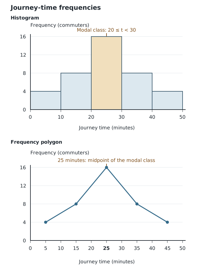
The histogram spans class boundaries; the frequency polygon places each frequency at a class midpoint.
The tallest rectangle and highest polygon point both identify minutes as the modal class. This does not reveal the exact mode: the individual times within the class are unknown. Similarly, the midpoint marks the class, not the journey time of every commuter in it.
For a frequency polygon, join consecutive midpoints only. Do not join the last point back to the first, or extend the graph down to the horizontal axis unless a plotted class actually has frequency zero.
When comparing two distributions, a peak further to the right suggests a higher modal value. Frequencies spread across a wider set of classes suggest more varied measurements. Grouping hides exact values, however, so it does not reveal the exact minimum, maximum or range. Direct comparisons of histogram heights require matching class intervals and frequency scales; also check whether the sample sizes match.
A distribution is positively skewed if its longer tail extends towards larger values. For example, many short journey times with a few much longer ones would produce a right-hand tail. A negatively skewed distribution has its longer tail towards smaller values.
An approximately symmetrical distribution has a similar shape on either side of its centre. The example journey-time frequencies above are symmetrical across their classes, although grouping does not tell us the exact arrangement of times within each class.
Describe skew using the tail, not simply the position of the tallest bar. When comparing graphs, explain what the shape means for the measurements in question.
Cumulative frequency is a running total. It answers questions such as ‘How many journey times are below 30 minutes?’ rather than ‘How many are between 20 and 30 minutes?’
Adding the journey-time frequencies gives:
| Journey time below, minutes | Cumulative frequency |
|---|---|
| 10 | 4 |
| 20 | 12 |
| 30 | 28 |
| 40 | 36 |
| 50 | 40 |
The total below 30 minutes is 28 because it includes all three classes below that boundary. Conversely, subtracting consecutive cumulative frequencies recovers a class frequency: the class contains commuters.
For grouped continuous data, plot cumulative frequency against each upper class boundary. By that boundary, the whole class has been counted. Start at the lowest class boundary with cumulative frequency zero; here that is . Label both axes, choose suitable scales and join the points with an increasing curve or consecutive straight-line segments, following any instruction in the question.
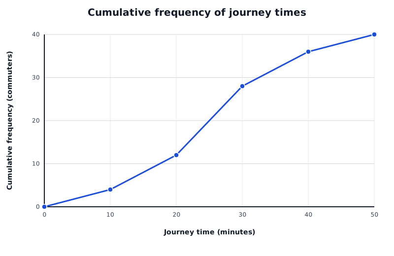
Each point counts all journeys below that upper class boundary. The final total is 40 commuters.
Data for Cumulative frequency of journey times
| Series | Journey time (minutes) | Cumulative frequency (commuters) |
|---|---|---|
| Journey times | 0 | 0 |
| Journey times | 10 | 4 |
| Journey times | 20 | 12 |
| Journey times | 30 | 28 |
| Journey times | 40 | 36 |
| Journey times | 50 | 40 |
The graph cannot fall: adding another frequency cannot reduce the running total. Its final cumulative frequency is the number of observations, here 40. A steep section means many observations lie within a relatively short interval of the horizontal scale.
To estimate how many observations lie below a particular measurement, start at that measurement on the horizontal axis, move vertically to the graph, then horizontally to the cumulative frequency axis.
The example gives 36 journeys below 40 minutes. Subtracting from the total shows that 4 journeys lasted at least 40 minutes. To find the number between two boundaries, subtract their cumulative frequencies: journeys lasted from 20 minutes up to, but not including, 40 minutes.
The median divides ordered data into two halves. The lower quartile, , marks about one quarter of the way through the data, and the upper quartile, , marks about three quarters of the way through it. For a grouped cumulative frequency chart containing observations, use these cumulative frequency levels:
From each level on the vertical axis, move horizontally to the graph, then vertically down to read the measurement. The vertical-axis number is a position in the data; the horizontal-axis reading is the quartile or median itself.
For the 40 commuters, use levels 10, 20 and 30. On the straight-line graph, these give estimated times of 17.5, 25 and 32.5 minutes respectively. The estimated median means about half the journeys were shorter than 25 minutes and half longer.
These are estimates because we do not know how the observations are distributed within each class. Straight segments assume an even spread within the interval. The interquartile range is the upper quartile minus the lower quartile, so the middle half of these journey times spans about 15 minutes.
For discrete data, cumulative frequency changes only when a possible data value is reached. A cumulative frequency step polygon shows this with vertical jumps and horizontal sections, rather than sloping lines between values.
For the books-read example, the cumulative frequencies at 0, 1, 2 and 3 books are 3, 8, 12 and 14.
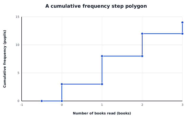
The cumulative total jumps at each possible number of books. Each jump height equals that value's frequency.
Data for A cumulative frequency step polygon
| Series | Number of books read (books) | Cumulative frequency (pupils) |
|---|---|---|
| Books read | -0.5 | 0 |
| Books read | 0 | 0 |
| Books read | 0 | 3 |
| Books read | 1 | 3 |
| Books read | 1 | 8 |
| Books read | 2 | 8 |
| Books read | 2 | 12 |
| Books read | 3 | 12 |
| Books read | 3 | 14 |
Start with cumulative frequency zero before 0 books. At 0, draw a vertical jump to 3, then a horizontal section to 1. At 1, jump from 3 to 8. Continue with a jump to 12 at 2 and a jump to 14 at 3. Each jump has a height equal to the frequency at that value.
The horizontal sections do not imply that pupils read fractional numbers of books. They show that no additional observations are counted between possible values.
At most 1 book includes both 0 and 1, so it accounts for 8 pupils. Fewer than 1 book includes only 0, so it accounts for 3. With 14 ordered observations, the median is found from the 7th and 8th values; both are 1 book, so the median is 1 book. Discrete readings come from the counted values, not by interpolating between steps.
A box plot summarises a distribution rather than showing every frequency. In a simple box plot, the whisker ends show the minimum and maximum, the box runs from to , and the line inside the box marks the median. If outliers are shown separately, check what the whisker ends represent.
The box contains the middle 50% of observations. Its length represents the interquartile range:
The overall range is the maximum minus the minimum. IQR focuses on the middle half and is less affected by extreme observations than the range.
Suppose two routes have these journey-time summaries, all in minutes:
| Route | Minimum | Median | Maximum | ||
|---|---|---|---|---|---|
| A | 5 | 18 | 25 | 32 | 50 |
| B | 10 | 22 | 28 | 34 | 42 |
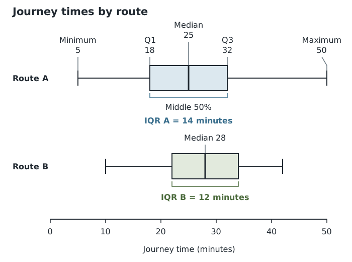
Route A has a lower median but a larger IQR: typical journeys are shorter, while the middle half of journey times is less consistent.
Route A has the lower median, 25 minutes compared with 28 minutes, suggesting a shorter typical journey. But its IQR is 14 minutes compared with 12 minutes for B, so the middle half of A's journey times is more spread out. Its range is also larger: 45 minutes compared with 32 minutes. Route B therefore appears more consistent, even though its median journey is longer.
For clues about shape, examine both halves of the box and the whiskers. A median nearer , together with more spread towards larger values, suggests positive skew; the reverse suggests negative skew. These are clues from a summary, not a full picture of the distribution. A centred median alone does not prove symmetry or a normal distribution.
A useful comparison combines a measure of typical value with a measure of spread, then explains both in context. For box plots, median and IQR are particularly useful. Neither a higher median nor a smaller spread is automatically ‘better’: the judgement depends on what the measurements represent.
Running total of frequencies; the final total is .
For grouped charts, read across to the graph and down from:
Grouped readings are estimates; discrete step readings use the actual possible values.
Read the median, quartiles and whisker ends; check whether outliers are separate.
Compare medians for typical values and IQRs for the spread of the middle 50%. Smaller IQR means greater consistency in that middle half. Support comparisons with numbers and interpret them in context.
Check both axis scales and units before comparing graphs. Raw frequencies can be misleading when the groups contain different numbers of observations.
Frequency polygons use class midpoints; grouped cumulative frequency charts use upper class boundaries.
On a discrete cumulative frequency step polygon, distinguish ‘less than’ from ‘at most’: at most includes the frequency at that value.
Give comparisons in context, supported by values: state which group has the higher average and which has the greater spread.
A box plot does not show the mean, mode or individual frequencies. Do not infer these from the box.
Quartiles read from a grouped cumulative frequency chart are estimates. Keep reading lines clear and include the units of the original variable.
It can see this note and what your specification asks for.
Answers are free with an account.
1 free note left this week
Get more free notesYour answer sets when this note comes back for review, or marks it complete.
Was this note helpful?
Log in to tell us whether it helped, or to report a problem.
Last updated
Frequency
The number of observations having a particular value or belonging to a particular category or class.
Bar line chart
A graph showing the frequency of each discrete numerical value using a separate vertical line.
Frequency polygon
A graph formed by plotting each class frequency against its class midpoint and joining consecutive points with straight lines.
Histogram
A graph of grouped continuous data using rectangles whose areas represent frequencies. With equal class widths, frequencies can be shown directly by bar heights on a frequency scale.
Cumulative frequency
The running total of frequencies up to a specified value or class boundary.
Cumulative frequency step polygon
A cumulative frequency graph for discrete data, with vertical jumps at possible data values and horizontal sections between them.
Box plot
A diagram summarising a distribution using its median, lower and upper quartiles, and the values shown at the whisker ends.
Lower quartile
The value separating approximately the lowest quarter of ordered data from the remaining three quarters.
Upper quartile
The value separating approximately the lowest three quarters of ordered data from the highest quarter.
Interquartile range
The spread of the middle 50% of the data, calculated as .
Skewness
Asymmetry in a distribution, usually described by the direction of its longer tail.
Put your knowledge into practice — try past paper questions for Statistics
Frequency
The number of observations having a particular value or belonging to a particular category or class.
Bar line chart
A graph showing the frequency of each discrete numerical value using a separate vertical line.
Frequency polygon
A graph formed by plotting each class frequency against its class midpoint and joining consecutive points with straight lines.
Histogram
A graph of grouped continuous data using rectangles whose areas represent frequencies. With equal class widths, frequencies can be shown directly by bar heights on a frequency scale.
Cumulative frequency
The running total of frequencies up to a specified value or class boundary.
Cumulative frequency step polygon
A cumulative frequency graph for discrete data, with vertical jumps at possible data values and horizontal sections between them.
Box plot
A diagram summarising a distribution using its median, lower and upper quartiles, and the values shown at the whisker ends.
Lower quartile
The value separating approximately the lowest quarter of ordered data from the remaining three quarters.
Upper quartile
The value separating approximately the lowest three quarters of ordered data from the highest quarter.
Interquartile range
The spread of the middle 50% of the data, calculated as .
Skewness
Asymmetry in a distribution, usually described by the direction of its longer tail.
| 15 |
| 16 | 25 |
| 8 | 35 |
| 4 | 45 |