

Loading…
Loading…
Loading…
AQA GCSE Statistics · 8382
AQA 8382 · 3.3.3 Constructing and Interpreting Charts and Graphs Check the specification (PDF) (opens in a new tab)
A histogram displays continuous numerical data grouped into class intervals. The horizontal axis shows the measured variable, such as time in minutes. Each bar extends from the lower boundary to the upper boundary of its class, so neighbouring classes have touching bars.
With unequal class widths, using frequency as the height would give wider classes disproportionately large bars. Instead, the area of each bar represents its frequency. A wide bar containing six observations must have the same area as a narrow bar containing six observations, so it must be shorter.
The height needed to make this work is called frequency density: the frequency per unit of class width. It describes how concentrated the observations are within the interval, rather than simply how many observations the interval contains.
Because a rectangle’s area is its width multiplied by its height:
Rearranging gives:
Consider these grouped times spent watching a television channel on one day. The interval includes 100 minutes but excludes 200 minutes, which belongs in the next class.
| Viewing time, (minutes) | Frequency | Class width (minutes) | Frequency density |
|---|---|---|---|
| 6 | 100 | 0.06 | |
Find each width by subtracting the lower boundary from the upper boundary. For example, the fourth class has width minutes, so its density is observations per minute.
The first and last classes both contain six observations. Their densities are different because those observations are spread across intervals of different widths: , but .
Choose a horizontal scale that accommodates all the class boundaries, from 0 to 800 minutes. The spacing must reflect numerical distance: the interval from 500 to 800 needs three times the width of the interval from 0 to 100.
Label the vertical axis Frequency density and choose a scale that accommodates the largest density, 0.36. Draw each rectangle across its complete class interval, with its height equal to the calculated density.
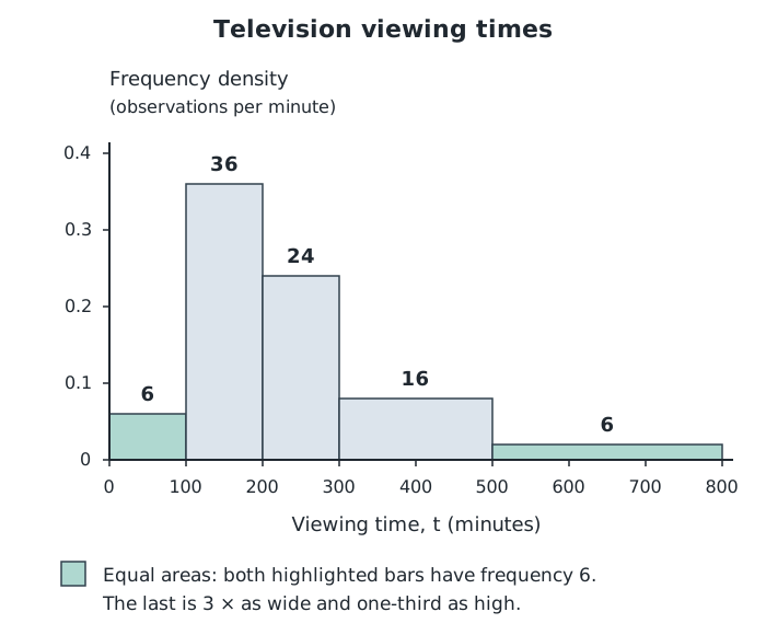
Frequency is represented by area. The first and last bars both represent six people, although their widths and heights differ.
The last bar is three times as wide as the first but only one-third as high. Their areas are therefore equal, correctly representing six people in each class.
To complete a partly drawn histogram, use exactly the same method: calculate the missing class’s width and density, then draw the rectangle between its boundaries using the existing axis scales.
To read a frequency, multiply the bar’s width by its density. The bar from 300 to 500 minutes has frequency , not 0.08.
Adding all the bar areas gives the total number of observations:
You can also estimate how many observations lie in part of a class. For example, to estimate how many people watched for more than 400 minutes, take the part from 400 to 500 and the whole final class:
This is about of the group. It is an estimate because taking part of a bar assumes that observations are evenly distributed within that class. The grouped data do not tell us their exact positions.
The median divides the histogram’s total area into equal halves. With 88 observations, locate the point with a frequency of to its left.
The first two bars contain observations, so the median lies in the class from 200 to 300 minutes. We need an additional frequency of within that bar.
Its density is 0.24, so the required horizontal distance into the bar is minutes. The estimated median is therefore minutes. Again, this assumes an even distribution within the class.
When comparing histograms, check the class intervals and axis scales before comparing their shapes. Matching intervals and density scales allow direct visual comparison, but frequencies still come from areas. If the groups have different totals, use proportions rather than raw frequencies to compare how common a range of values is.
For example, suppose a second group of 88 people has frequencies of 18, 36, 18, 12 and 4 in the same five viewing-time classes. Its first two classes contain people, so its median lies between 100 and 200 minutes. The original group’s median lies between 200 and 300 minutes. This supports the conclusion that the second group typically spent less time watching the channel.
The second group also has fewer people watching for at least 300 minutes: , compared with in the original group. Both groups have observations in the same lowest and highest classes, however, so these grouped data do not establish their exact ranges.
Calculate each class width from its boundaries, then write down the frequency density before drawing the bar.
For unequal-width histograms, compare bar areas to compare frequencies: the tallest bar need not contain the most observations.
Read both axis scales carefully. A square on the grid does not necessarily represent one unit.
When estimating a frequency within part of a class, state that you assume the observations are evenly distributed within that class.
Support comparisons with values or proportions, not just statements such as ‘the bars look higher’.
It can see this note and what your specification asks for.
Answers are free with an account.
1 free note left this week
Get more free notesYour answer sets when this note comes back for review, or marks it complete.
Was this note helpful?
Log in to tell us whether it helped, or to report a problem.
Last updated
Histogram
A graph of grouped continuous data in which each bar spans a class interval and its area represents the frequency.
Class interval
A range used to group numerical observations, such as minutes.
Class width
The upper class boundary minus the lower class boundary.
Frequency
The number of observations in a group or class interval.
Frequency density
The frequency per unit of class width, calculated using .
Put your knowledge into practice — try past paper questions for Statistics
Histogram
A graph of grouped continuous data in which each bar spans a class interval and its area represents the frequency.
Class interval
A range used to group numerical observations, such as minutes.
Class width
The upper class boundary minus the lower class boundary.
Frequency
The number of observations in a group or class interval.
Frequency density
The frequency per unit of class width, calculated using .
| 36 |
| 100 |
| 0.36 |
| 24 | 100 | 0.24 |
| 16 | 200 | 0.08 |
| 6 | 300 | 0.02 |