

Loading…
Loading…
Loading…
OCR GCSE Combined Science B · J260
OCR J260 · Non-Communicable Diseases Check the specification (PDF) (opens in a new tab)
Disease data help scientists identify patterns, investigate possible risk factors and assess prevention or treatment. Before interpreting a figure, establish exactly what has been counted, which population it describes and the period covered.
Incidence counts new cases during a stated period. For example, the number of people newly diagnosed with a disease during one year describes its incidence. Prevalence counts people who have the disease at a particular time, including those diagnosed earlier. A treatment that helps people live longer with a disease could increase prevalence without increasing the number of new cases. Mortality describes deaths, rather than diagnoses.
Population size matters. Suppose one town records 100 new cases among 10,000 residents in a year, while another records 200 among 40,000 residents. The second town has more cases, but a smaller proportion of its residents develop the disease: 0.5%, compared with 1% in the first town. Comparisons should use the same time period and a common population basis, such as new cases per 100,000 people per year.
Non-communicable diseases do not pass directly from person to person. Their occurrence can differ between neighbourhoods, across a country and around the world. Exercise, diet, alcohol consumption and smoking can help explain disease patterns, but they are not the only influences.
Consider cardiovascular disease, which affects the heart and blood vessels. In Leicester, 33% of adults did less than 30 minutes of physical activity per week, compared with 22% in England. Only 27% of Leicester residents ate five portions of fruit or vegetables daily, compared with 33% in England. These patterns suggest that inactivity and unhealthy diet could contribute to cardiovascular disease risk locally.
However, not every lifestyle measure points in the same direction. Smoking was recorded for 13% of Leicester adults, similar to England overall, so this comparison alone does not suggest that a higher current smoking percentage explains Leicester's difference. Half of Leicester residents abstained from alcohol, although many drinkers consumed at least 14 units per week. An average or a statement about abstinence can therefore conceal differences within a population.
In 2021, Leicester's age-standardised cardiovascular mortality rate was 288.6 deaths per 100,000 people, compared with 230.4 for England. Age-standardisation makes comparisons fairer by allowing for different population age structures. The higher mortality rate is consistent with concern about local cardiovascular health; the activity and diet figures offer plausible contributing explanations, not proof of the cause of each death.
Cancer registrations record newly diagnosed cancers, so they provide incidence data rather than a count of everyone already living with cancer. During 2017–19, Leicester registered 580 lung cancer diagnoses and 174 oral cancer diagnoses. Lung cancer registration rates were significantly higher than England's. The oral cancer registration rate was 23 per 100,000 people, compared with 15 nationally.
Smoking is an important explanation to consider because it increases the risk of lung and oral cancers. Cancer-causing chemicals in tobacco smoke can damage cells, including those lining the lungs. The higher local registration rates are therefore consistent with smoking contributing to these disease patterns, although they do not show that every diagnosed person smoked.
The timing of lifestyle data matters. Leicester's adult smoking estimate was 13.1%, similar to England's 12.7%, but smoking among Leicester men had previously been higher than England's before falling to a similar level by 2021. A current smoking percentage does not describe people's past exposure. It therefore cannot, on its own, explain cancer diagnoses recorded in an earlier period.
Other influences also need considering. Lung cancer risk is affected by passive smoking and long-term exposure to air pollution, as well as factors such as family history. Differences in age and diagnosis can also affect recorded incidence. A justified explanation links the higher new-case rates to relevant risks while recognising that smoking is not the only possible influence.
Recorded coronary heart disease prevalence in 2021/22 was 2.3% in Leicester, compared with 3.0% in England. This is lower recorded prevalence alongside higher cardiovascular mortality, not a contradiction: the figures measure different things, and coronary heart disease is only one cardiovascular condition.
Age also matters. Just 28% of Leicester's population was over 50, compared with 39% in England. Because cardiovascular conditions become more common with age, a younger population can have lower overall prevalence. Recorded prevalence is also affected by diagnosis: undiagnosed illness will not appear in a register of diagnosed cases.
The useful conclusion is therefore qualified: Leicester has some less favourable lifestyle patterns and higher cardiovascular mortality, but its younger population and differences in diagnosis help explain why recorded prevalence need not follow the same pattern. Cancer registrations add information about new diagnoses; prevalence and mortality describe different aspects of the health picture. No single percentage summarises them all.
In England in 2022, there were 41,713 new lung cancer registrations, compared with 39,933 bowel cancer registrations. Prostate cancer was the most commonly diagnosed cancer, with 54,732 new diagnoses. Excluding two common types of non-melanoma skin cancer, prostate, breast, lung and bowel cancers together accounted for 51% of registered cancer diagnoses.
The large number of new lung cancer diagnoses makes smoking an important national risk factor to investigate. In the United Kingdom in 2016, current tobacco smoking was recorded for 21% of people aged 15 and over. This indicates that exposure to a known lung cancer risk factor was widespread, but it is not a measurement of smoking among the people diagnosed in England in 2022. The population and year differ, and passive smoking, air pollution and other causes also contribute to lung cancer.
Other national lifestyle figures help identify prevention priorities. In the UK in 2016, physical inactivity was recorded for 38% of adults aged 18 and over, and obesity for 30% of adults aged 18 and over. Mean salt intake was 9 g per day for adults aged 20 and over in 2010. Alcohol consumption averaged 11 litres of pure alcohol per person aged 15 and over in 2016; this is pure alcohol, not the volume of alcoholic drinks.
Smoking, unhealthy diet, physical inactivity and alcohol consumption are risk factors for cancer and other non-communicable diseases. Reducing smoking and alcohol consumption, being regularly active and eating a healthy diet can reduce risk. For lung cancer prevention, this includes quitting smoking, exercising regularly and eating at least five portions of fruit and vegetables daily. These actions reduce risk rather than guaranteeing that disease will not develop.
Recorded incidence can also change because more cancers are detected. A prostate cancer awareness campaign in England in 2022 encouraged men to check their risk and was followed by an all-time high number of urgent suspected-cancer referrals in March. Increased awareness and testing can raise registrations without a corresponding change in lifestyle. A rise in recorded diagnoses should therefore not automatically be blamed on worsening behaviour.
The national lifestyle percentages should not be compared directly with every Leicester percentage: the years, age groups and definitions differ. In particular, ‘physical inactivity’ is not automatically the same measure as ‘less than 30 minutes of activity per week’.
Worldwide in 2024, the most common cancers by number of new cases were lung cancer, with 2.6 million cases; breast cancer, with 2.4 million; colon and rectum cancers, with 2.0 million; and prostate cancer, with 1.5 million. These figures describe incidence. They show that lung cancer had the largest new-case total among these cancers, but raw worldwide totals cannot be compared directly with the totals for a city or country.
Tobacco use is an important explanation for lung cancer's global burden, while air pollution is another important risk factor. Across cancers more broadly, alcohol consumption, unhealthy diet, physical inactivity and high body mass index also contribute to risk. Nearly a quarter of cancer deaths worldwide are linked to tobacco use, alcohol consumption, high body mass index, low fruit and vegetable intake, and lack of physical activity. That fraction describes deaths, not the fraction of new diagnoses caused by those factors.
Cancer incidence rises sharply with age, partly because exposure to risk factors accumulates over a lifetime. Consequently, differences between populations may reflect age structure as well as lifestyle. Access to diagnosis also influences how many cases are recorded. Lifestyle prevention is nevertheless important worldwide: approximately 38% of cancers can currently be prevented by avoiding risk factors and using established prevention strategies.
Mortality figures provide a different perspective. Non-communicable diseases accounted for an estimated 89% of UK deaths in 2016, compared with 71% globally. Worldwide, this represented about 41 million deaths, including 17.9 million from cardiovascular disease and 9 million from cancer. These are proportions and numbers of deaths, not the proportions of people developing a disease.
The higher UK share of deaths from non-communicable diseases does not establish that every UK lifestyle factor is worse than the global average: population age and the frequency of other causes of death also affect the percentage.
At any scale, build an explanation in the same order: identify what was measured, describe the pattern with figures, link relevant lifestyle factors, and consider other explanations. Income and location can influence access to food and healthcare, so lifestyle differences should not automatically be treated as unrestricted individual choices. A national average can also conceal large local differences.
A table preserves individual numerical values; a graph makes an overall pattern easier to see. Choosing the right graph depends on what the values represent, whether they concern disease causes, spread, effects or treatment.
Consider this teaching example of monthly measles cases:
| Month | New cases |
|---|---|
| January | 8 |
| February | 15 |
| March | 22 |
| April | 25 |
| May | 18 |
| June | 10 |
To construct a bar chart, place the months in chronological order on the horizontal axis and label the vertical axis ‘Number of new cases’. Use an evenly spaced scale starting at zero and extending beyond 25. Draw equal-width, separated bars with heights matching the table.
To convert the chart back into numerical form, read each bar against the vertical scale and enter its value beside the correct month. The pattern is an increase from 8 cases in January to a peak of 25 in April, followed by a decrease to 10 in June. Simply saying ‘cases increased’ would miss the later decline.
The same method works for non-communicable disease diagnoses, categories of treatment or disease deaths. Keep the original meaning in the axis label: a bar showing deaths must not be relabelled as new cases.
Frequency means how many observations belong to a category or interval. A frequency table can summarise diagnoses by disease category, or group continuous measurements such as patients’ ages into intervals.
Suppose the ages, in years, of ten patients are 22, 24, 28, 31, 35, 37, 39, 42, 45 and 48. Count each patient once in the appropriate interval:
| Age interval / years | Frequency |
|---|---|
| 3 | |
| 4 | |
| 3 |
Here, represents age. The boundaries do not overlap: someone aged exactly 30 belongs in the second interval. Adding the frequencies gives ten, matching the original number of patients.
A histogram displays continuous data grouped into intervals. Put age on the horizontal axis and frequency on the vertical axis. For these equal-width intervals, draw touching bars of heights 3, 4 and 3. The touching bars show that the age scale is continuous, unlike the separate categories in a bar chart. The largest frequency is in the 30–under-40 interval, but the histogram no longer reveals each individual age.
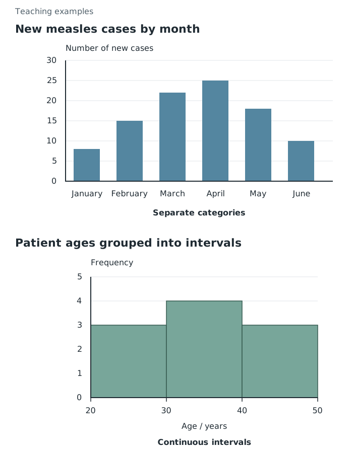
Separated bars compare months; touching histogram bars group ages into continuous intervals.
Scientists often cannot collect information from everyone in a population. A sample saves time and resources while allowing them to investigate disease patterns in a smaller group.
The sample should represent the population relevant to the question. To investigate adult health across a town, collecting responses only from members of a gym would probably over-represent physically active adults. Increasing the number of gym members surveyed would not remove that selection bias.
Random selection gives individuals an equal chance of selection and reduces deliberate selection bias. Researchers should also check that relevant groups, such as different ages and neighbourhoods, are adequately represented. A larger, well-chosen sample is generally less affected by chance differences than a small one. However, people who do not respond may differ from those who do, so the final sample still needs checking.
Use consistent definitions and collection methods: for example, ask everyone about exercise over the same period and use the same criteria for identifying disease. Conclusions from one narrow group should not automatically be extended to the whole country or world.
A scatter diagram plots paired values for two variables. Each point might represent one town, with its air pollution level on the horizontal axis and its number of asthma cases on the vertical axis. Plot each pair at its corresponding horizontal and vertical coordinates; do not join the towns as though they form a time sequence.
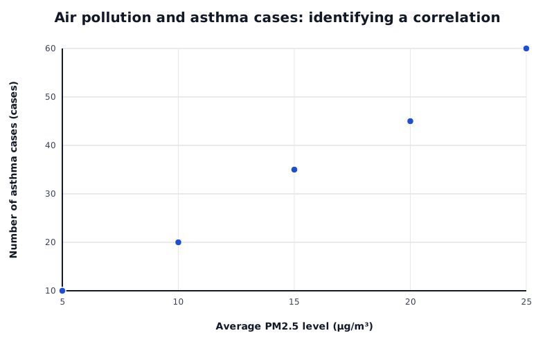
Each point represents a town in a teaching example. The upward pattern shows a positive correlation, not proof of causation.
Data for Air pollution and asthma cases: identifying a correlation
| Series | Average PM2.5 level (µg/m³) | Number of asthma cases (cases) |
|---|---|---|
| Towns | 5 | 10 |
| Towns | 10 | 20 |
| Towns | 15 | 35 |
| Towns | 20 | 45 |
| Towns | 25 | 60 |
Read the pattern from left to right. An upward trend is a positive correlation: higher values of one variable tend to occur with higher values of the other. A downward trend is a negative correlation. If the points show no clear upward or downward pattern, there is no clear correlation.
In this teaching example, asthma cases generally increase as air pollution increases. At 5 µg/m³ there are 10 cases, compared with 60 cases at 25 µg/m³. These figures support a positive association, not proof that pollution alone caused the difference.
Another factor might affect both variables, and towns with larger populations might have more asthma cases simply because more people live there. A stronger investigation would compare cases on a common population basis and consider other relevant factors. Scatter diagrams help identify relationships worth investigating; establishing causation requires further evidence.
Use a sufficiently large, representative sample. Random selection reduces selection bias; check relevant groups and non-response. Keep collection methods consistent. Size alone does not remove bias.
Plot paired values for two variables.
Describe both variables and support the pattern with figures. Correlation does not prove causation.
Check whether the figures count new cases over a stated period, all existing cases or deaths. Incidence, prevalence and mortality are not interchangeable.
When comparing populations, use figures for the same population size and time period rather than comparing raw totals alone.
Describe a pattern using both variables, then support it with figures from the data.
A correlation suggests an association; it does not, by itself, prove that one variable causes the other.
Use separated bars for categories and touching bars for continuous class intervals. Label axes and include units where appropriate.
A large sample can still be biased: explain how participants were selected as well as how many were included.
Check the age group, year and definition of a lifestyle measure before comparing percentages from different datasets.
It can see this note and what your specification asks for.
Answers are free with an account.
1 free note left this week
Get more free notesYour answer sets when this note comes back for review, or marks it complete.
Was this note helpful?
Log in to tell us whether it helped, or to report a problem.
Last updated
Incidence
The number of new cases of a disease in a population during a stated period.
Prevalence
The number or proportion of people in a population who have a disease at a particular time.
Mortality
Deaths in a population, often expressed as a rate over a stated period.
Frequency table
A table recording how many observations fall into each category or interval.
Bar chart
A graph with separated bars used to compare frequencies or values for distinct categories.
Histogram
A graph showing the frequency distribution of continuous data grouped into intervals, with touching bars.
Sample
A smaller group selected from a population to collect information about that population.
Representative sample
A sample that reflects the relevant characteristics of the population being investigated.
Bias
A systematic distortion in data collection or selection that can make results unrepresentative.
Scatter diagram
A graph in which each point represents a pair of values for two variables.
Correlation
An association between two variables, shown by a pattern in their values.
Causation
A relationship in which a change in one factor produces a change in another.
Put your knowledge into practice — try past paper questions for Combined Science B
Incidence
The number of new cases of a disease in a population during a stated period.
Prevalence
The number or proportion of people in a population who have a disease at a particular time.
Mortality
Deaths in a population, often expressed as a rate over a stated period.
Frequency table
A table recording how many observations fall into each category or interval.
Bar chart
A graph with separated bars used to compare frequencies or values for distinct categories.
Histogram
A graph showing the frequency distribution of continuous data grouped into intervals, with touching bars.
Sample
A smaller group selected from a population to collect information about that population.
Representative sample
A sample that reflects the relevant characteristics of the population being investigated.
Bias
A systematic distortion in data collection or selection that can make results unrepresentative.
Scatter diagram
A graph in which each point represents a pair of values for two variables.
Correlation
An association between two variables, shown by a pattern in their values.
Causation
A relationship in which a change in one factor produces a change in another.