

Loading…
Loading…
Loading…
Eduqas GCSE Geography B · C112
Eduqas C112 · 3.1 Check the specification (PDF) (opens in a new tab)
Interpret and analyze atlas maps, topological maps, and Ordnance Survey maps at various scales (1:50,000 and 1:25,000).
Analyze contour lines, spot heights, and gradients to understand terrain profiles.
Evaluate isoline maps, such as weather synoptic charts and ocean bathymetric charts.
Interpret maps featuring proportional symbols to understand geographical data distribution.
A map represents selected information about places. Its title tells you what it shows, its key explains the symbols or colours, and its scale connects distances on the page to distances on the ground. Start with these before interpreting a pattern: a colour might represent height on one map but population on another.
An atlas contains maps covering different areas and themes. Physical maps show features such as mountains, rivers and seas; political maps show boundaries and cities; thematic maps focus on a particular variable, such as rainfall or population. Relief means the height and shape of the land, while drainage describes its rivers and other water bodies.
To analyse an atlas map, identify the broad pattern, compare areas and support your description with the key. Suppose a height key places one area in a 0–200 m band and another in a 600–1,000 m band. You can conclude that the second area is generally higher, but you cannot obtain an exact summit height from those bands. Comparing a relief map with a drainage map can help you investigate how rivers relate to the shape of the land.
Ordnance Survey maps show detailed physical and human features of Great Britain. Read their symbols using the map’s key, then combine features rather than treating each symbol separately: roads, buildings, watercourses and relief together help you understand a landscape.
A scale of 1:25,000 means that one unit on the map represents 25,000 of the same units on the ground. Therefore, 1 cm represents 25,000 cm, or 250 m. At 1:50,000, 1 cm represents 500 m.
For example, suppose two points are 4 cm apart on a printed map. At 1:25,000 their straight-line separation is 1 km; at 1:50,000 it is 2 km. The printed distance alone is not enough to determine the ground distance.
The 1:25,000 map is the larger-scale map: it shows a smaller area in greater detail for the same-sized sheet. A 1:50,000 map provides a wider overview. This distinction matters when comparing maps: a feature may be omitted or simplified on the smaller-scale map without being absent from the landscape. The same principle applies to atlas maps: a world map provides a broad overview, while a larger-scale national or regional map can show finer detail.
For a straight-line distance, measure between the points with a ruler and convert using the scale. For a winding route, follow its bends with a strip of paper or thread, then measure the total length. Use the scale bar if the image has been resized, because a stated ratio only applies at the intended printed size.
A topological map shows how places connect within a network. Unlike a topographical map, which represents the landscape and its relief, it can distort distances, directions and shapes to make connections easier to read.
The London Underground map is a familiar example. It preserves the order of stations and shows where lines meet, allowing passengers to identify where to board, leave or change trains. The drawn distance between stations is not a reliable measure of their separation on the ground.
Suppose one line connects stations A–B–C and another connects D–B–E. To travel from A to E, follow the first line to B, change there, and follow the second line to E. B is the interchange because both lines connect there. This reasoning transfers to real transport maps: trace the connected lines and station order, checking that a crossing is marked as an interchange. The map can establish a route, but equal-looking gaps between stations do not establish equal distances or journey times.
A contour joins points at the same height above sea level. On OS maps, contours are brown. Imagine marking the edge of water around a hill as the water level falls by equal amounts: each mark would trace another contour.
The contour interval is the vertical difference between neighbouring contours. On 1:25,000 OS maps it is usually 5 m, although it may be 10 m in mountainous areas. Check the map information. Where some contours are unlabelled, count the intervals between labelled lines to work out their heights.
Contour spacing reveals steepness. Closely spaced contours show a large height change over a short horizontal distance, so the slope is steep. Widely spaced contours show the same height change spread over a longer distance, so the slope is gentle. Successively higher closed contours indicate rising ground towards a hilltop.
A spot height gives the height of one particular point. It adds precision that contours cannot always provide. For example, a summit inside a 140 m contour might have a spot height of 147 m: the contour shows the surrounding shape, while the spot height gives the summit’s elevation.
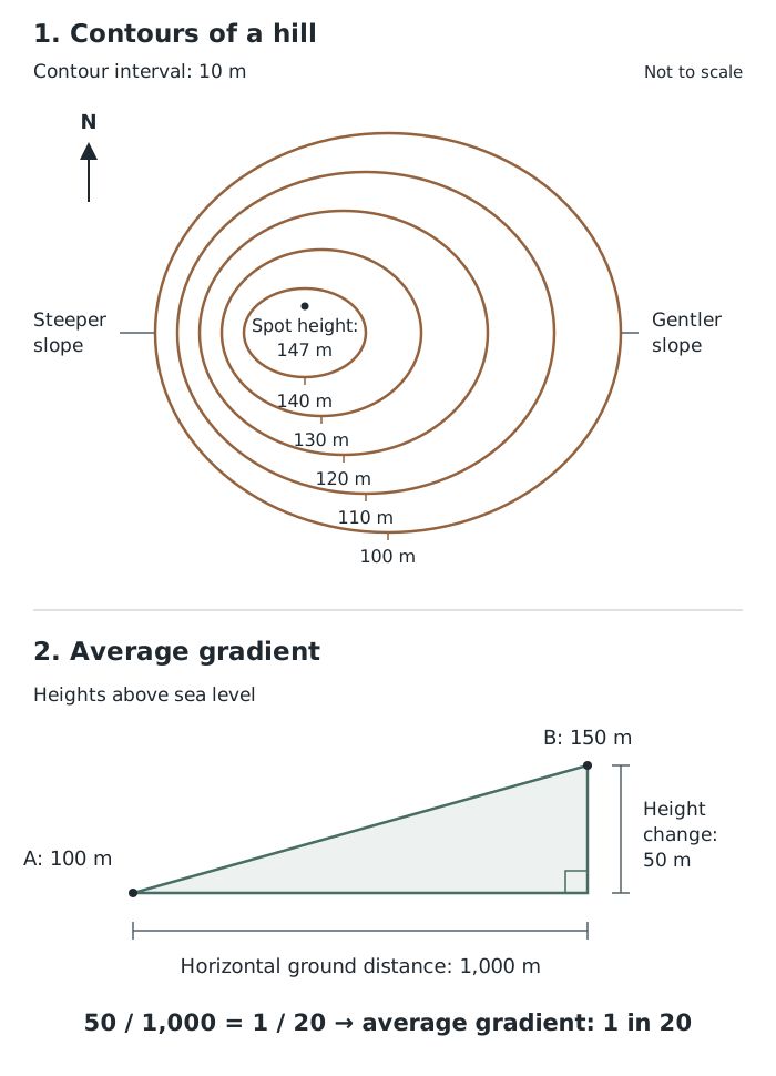
Contour spacing shows differences in steepness; gradient compares height change with horizontal distance. This example uses a 10 m contour interval.
In the hill sketch, compare the two sides. Each crosses the same sequence of heights, but the contours are closer together on the western side. That side is therefore steeper. The spot height identifies the summit’s height rather than the height of the entire enclosed area. Apply the same reasoning to an OS map, using its own contour interval and scale.
Gradient compares the vertical change in height with the horizontal ground distance. It describes the average steepness between two points rather than every small change along the slope.
Suppose point A is 100 m above sea level and point B is 150 m above sea level. Their horizontal separation is 1,000 m. The height change is m, so the gradient is , usually written 1 in 20. This means a vertical change of 1 m for every 20 m horizontally.
For comparison, a gradient of 1 in 10 is steeper: the same 1 m height change occurs over only 10 m horizontally. A route can also vary in steepness, so use contour spacing to identify particularly steep sections rather than relying only on its average gradient.
Contours are one type of isoline. Other isolines join places with equal values of other variables. Before interpreting them, establish what is measured, its unit and the period represented. Rainfall measured over 12 hours is not the same quantity as annual rainfall.
A rainfall example covering a 12-hour period has readings of about 6.7–7.0 mm near its centre, compared with readings of 0.3–0.7 mm near the upper edge. The readings and surrounding isolines indicate a broadly concentric pattern, with higher rainfall towards the centre and lower rainfall towards the outskirts.
Describe that pattern before suggesting a cause. A land-use map could help investigate whether vegetation affected the amounts collected: trees can intercept rainfall before it reaches a rain gauge. However, the rainfall pattern alone does not establish that vegetation caused it. Additional evidence is needed to test an explanation.
Isolines also estimate how a variable changes between observations. More observations can reveal detail that a sparse set of measurements misses, so avoid treating every mapped boundary as an exact measurement at every point.
A synoptic chart shows weather conditions across an area at a particular time. Its isobars join places with equal atmospheric pressure, usually measured in hectopascals (hPa). Some charts use millibars (mb), which have the same numerical value. Check the date and time before using a chart to describe conditions.
Follow the pressure values towards the centre of a system. Values increasing inwards indicate an anticyclone, or high-pressure system; values decreasing inwards indicate a depression, or low-pressure system. Closed isobars help reveal their centres.
Isobar spacing gives evidence about wind strength. Closely spaced isobars mean that pressure changes rapidly over a short distance: this is a steep pressure gradient and is associated with stronger winds. Widely spaced isobars indicate a gentler pressure gradient and lighter winds. Compare spacing where the pressure intervals and map scale are the same.
Wind blows almost parallel to the isobars. In the Northern Hemisphere, including the UK, winds circulate clockwise around an anticyclone and anticlockwise around a depression. These directions are reversed in the Southern Hemisphere. Isobars therefore help you infer both relative wind strength and the general direction of airflow, but their spacing alone does not give an exact wind speed.
A front is a boundary between air masses with different temperatures. On a synoptic chart, fronts are thicker lines carrying distinctive symbols:
The triangles and semicircles point in the direction the front is moving. Use the front’s position and movement to reason about weather changes at a place, rather than assuming the whole map area has the same weather.
For example, a place just ahead of an approaching active cold front may experience rain as it passes and colder, brighter or showery weather afterwards. If the surrounding isobars are close together, strong winds are also likely. These are reasoned expectations, not guarantees: weak fronts may bring little or no rain, and weather changes can be less marked.
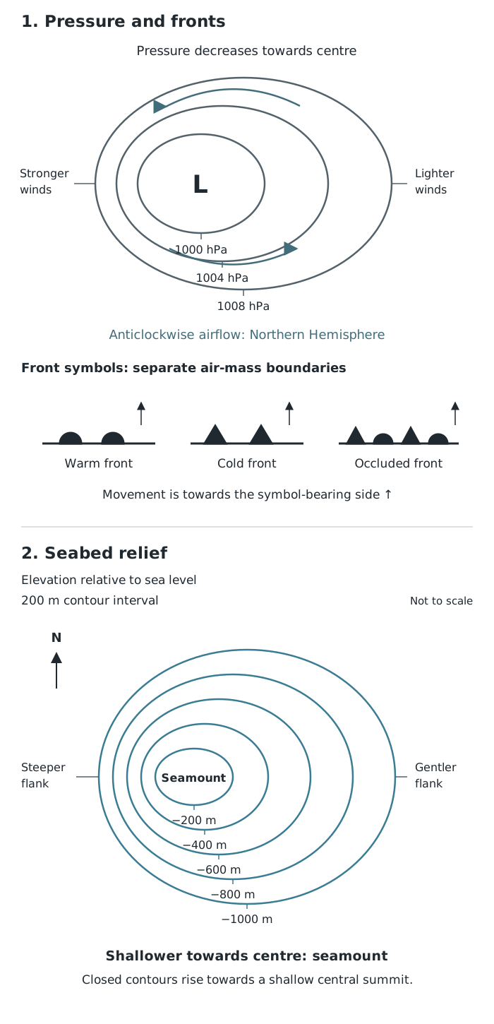
Read the values as well as the shapes: isobars identify pressure systems, while depth contours reveal seabed relief.
The pressure panel demonstrates how values identify a low-pressure centre and how spacing identifies relatively stronger winds. The front symbols are separate from the isobars: they show air-mass boundaries, not equal pressure.
A bathymetric chart shows the depth and shape of the seabed. Its depth contours join places at equal depth below sea level. Read the units and labelling convention first: depth may be expressed as metres below sea level or as a negative elevation. For example, −200 m is 200 m below sea level and is shallower than −1,000 m.
The same spacing principle used on land applies underwater. Closely spaced depth contours indicate a steep seabed slope; widely spaced contours indicate a gentler slope. To recognise an underwater hill, or seamount, look for closed contours that become shallower towards the centre. Closed contours becoming deeper inwards instead indicate a depression. The values, not the closed shape alone, determine which it is.
In the seabed panel, the contours change from −1,000 m outside to −200 m towards the centre. The seabed therefore rises towards a shallow central summit. Its western flank is steeper because the same depth intervals are closer together there. This is a constructed example; on an ocean chart, apply the method using that chart’s own depth interval and scale.
Colour can also represent depth, but its meaning comes from the key, not from the colour itself. Resolution is the amount of detail a map can reveal. Low-resolution seabed mapping provides a broad picture but may miss small features, such as craters. Higher-resolution multibeam sonar mapping reveals finer seabed relief. A large printed image does not necessarily contain detailed underlying observations, so judge whether the chart is suitable for the feature you are investigating.
A proportional-symbol map places symbols on a base map and varies their size according to a quantity. The positions show where the data belong; the sizes show differences in value.
Read the title, units and symbol key first. Then identify the largest and smallest values, describe any clusters or contrasts, and look for exceptions. For example, a map of Human Development Index using 2018 data shows larger symbols for northern African countries such as Tunisia and Algeria than for Niger and Chad. That supports a comparison of the mapped development values, not a claim that the countries with larger symbols have larger populations or land areas.
Use the key to estimate values rather than judging size by eye alone. Overlapping symbols may hide smaller ones, and one symbol for a whole country cannot reveal differences within it. The map is useful for comparing places, but it does not by itself explain why their values differ.
Use matching units. 1 in 10 is steeper than 1 in 20. Gradient between two points is an average.
At 1:25,000, 1 cm represents 250 m; at 1:50,000, it represents 500 m. Convert distances before calculating gradient.
For gradient calculations, use the difference in height, not the height of the higher point, and put both distances in the same units.
Check the contour interval rather than assuming every map uses the same one.
Compare contour spacing on maps at the same scale: changing the scale also changes the printed spacing.
Use a proportional-symbol map’s key to interpret symbol sizes. Do not assume that doubling a circle’s diameter doubles its value.
Support a description of a distribution with values and locations, then distinguish the observed pattern from a possible explanation.
Topological maps show connections, not reliable ground distances. Do not use the length of a drawn transport line to calculate journey distance.
On synoptic charts, distinguish thin isobars from the thicker lines carrying front symbols. Check the chart’s date and time.
For bathymetric contours, check whether labels give positive depths or negative elevations: −200 m is shallower than −1,000 m.
It can see this note and what your specification asks for.
Answers are free with an account.
1 free note left this week
Get more free notesYour answer sets when this note comes back for review, or marks it complete.
Was this note helpful?
Log in to tell us whether it helped, or to report a problem.
Last updated
Map scale
The relationship between a distance on a map and the corresponding distance on the ground.
Relief
The height and shape of the land, including differences in elevation and slope.
Contour
A line joining points of equal height above sea level.
Contour interval
The vertical difference in height between neighbouring contour lines.
Spot height
The height above sea level of one particular point, usually labelled in metres.
Gradient
The steepness of a slope, calculated by comparing its vertical change in height with its horizontal distance.
Isoline
A line on a map joining places with an equal value of a particular variable, such as height or rainfall.
Proportional-symbol map
A map on which symbols placed at locations are sized in proportion to the quantities they represent.
Topological map
A map showing connections and the order of places within a network, while simplifying or distorting their distances, directions and positions.
Synoptic chart
A weather map showing atmospheric conditions over an area at a particular time, including pressure systems and fronts.
Isobar
A line joining places with equal atmospheric pressure.
Anticyclone
An area with higher atmospheric pressure at its centre than in its surroundings.
Depression
An area with lower atmospheric pressure at its centre than in its surroundings.
Front
A boundary between air masses with different temperatures.
Bathymetric chart
A map showing the depth and shape of the seabed.
Put your knowledge into practice — try past paper questions for Geography B
Map scale
The relationship between a distance on a map and the corresponding distance on the ground.
Relief
The height and shape of the land, including differences in elevation and slope.
Contour
A line joining points of equal height above sea level.
Contour interval
The vertical difference in height between neighbouring contour lines.
Spot height
The height above sea level of one particular point, usually labelled in metres.
Gradient
The steepness of a slope, calculated by comparing its vertical change in height with its horizontal distance.
Isoline
A line on a map joining places with an equal value of a particular variable, such as height or rainfall.
Proportional-symbol map
A map on which symbols placed at locations are sized in proportion to the quantities they represent.
Topological map
A map showing connections and the order of places within a network, while simplifying or distorting their distances, directions and positions.
Synoptic chart
A weather map showing atmospheric conditions over an area at a particular time, including pressure systems and fronts.
Isobar
A line joining places with equal atmospheric pressure.
Anticyclone
An area with higher atmospheric pressure at its centre than in its surroundings.
Depression
An area with lower atmospheric pressure at its centre than in its surroundings.
Front
A boundary between air masses with different temperatures.
Bathymetric chart
A map showing the depth and shape of the seabed.