Loading…


Loading…
Loading…
Loading…
AQA GCSE Combined Science Trilogy · 8464
AQA 8464 · 4.7.2.1 Levels of Organization and Trophic Relationships Check the specification (PDF) (opens in a new tab)
Understand that photosynthetic organisms serve as the primary producers of all biomass for life on Earth.
Describe how feeding relationships within a community are accurately represented by food chains, always beginning with a producer that synthesises molecules.
Explain that producers are typically green plants or algae that manufacture glucose through the process of photosynthesis.
Understand how ecologists utilise experimental methods, specifically transects and quadrats, to determine the precise distribution and abundance of species in an ecosystem.
Understand the mathematical terms mean, mode, and median in the context of analysing the abundance of organisms.
Calculate arithmetic means from ecological sampling data.
Plot and draw appropriate graphs by selecting appropriate scales for the axes based on biological data.
Explain the flow of energy from producers to primary consumers, followed by secondary and tertiary consumers.
Describe predators as consumers that actively kill and eat other animals, and identify the eaten animals as prey.
Understand that in a stable community, the numbers of predators and prey will rise and fall in predictable cycles.
Interpret graphs designed to mathematically model these predator-prey population cycles.
Evaluate methods for measuring the population size of a common species in a natural habitat.
Assess the effect of an environmental factor on the distribution of a species using appropriate sampling techniques.
A population consists of all the organisms of one species living in a particular habitat. Ecologists investigate both its abundance — how many individuals there are — and its distribution — where they occur. Two areas could contain similar numbers of daisies but have different distributions: daisies might be spread throughout one area and concentrated in patches in the other.
Counting every organism in a large habitat would often take too long. Instead, ecologists count organisms in smaller samples and use these to estimate abundance across the whole area. The estimate depends on how well the samples represent the habitat; it is not an exact census.
A quadrat is a frame enclosing a known area. It is suitable for plants and slow-moving animals because they are unlikely to move into or out of the sample during counting. For a clearly identifiable plant such as a daisy, count the individuals inside the frame. When individuals are difficult to distinguish, as with grass or moss, estimate percentage cover: the percentage of the quadrat occupied by that species. A subdivided quadrat helps you judge the area covered. Percentage cover measures abundance but does not directly give a number of individual plants.
The first part of AQA required practical activity 7 uses sampling to estimate the population size of a common species in a habitat. A suitable investigation is to count daisies in a grassed area.
You need a quadrat of known dimensions, tape measures or marked strings, a way to choose random coordinates, and a recording sheet on a clipboard. Quadrats measuring 25 cm × 25 cm or 50 cm × 50 cm are suitable examples. Identify the target species before starting so that everyone counts the same organism.
Random selection reduces bias: the person sampling does not deliberately choose patches with many daisies or places that are easiest to reach. Taking many samples helps capture differences between patches.
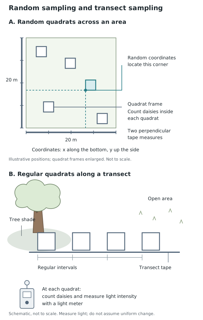
Random quadrats sample the whole area; quadrats along a transect reveal changes across a habitat.
First calculate the mean number of individuals per quadrat:
Then scale up according to how many quadrat-sized areas fit into the habitat:
Equivalently, multiply the total number counted by the total habitat area divided by the total area sampled.
For example, suppose 50 daisies are counted across ten 25 cm × 25 cm quadrat samples in a 20 m × 20 m survey area. Each quadrat has an area of , so the ten samples cover . The habitat area is .
This estimate assumes that the sampled density is representative of the whole survey area. It does not mean that exactly 32,000 daisies have been counted.
Random sampling is useful for estimating abundance across an area. To investigate how distribution changes across a habitat, use a transect: a line along which samples are taken. A line transect can record species touching the line; placing quadrats at regular intervals also records abundance in a known area beside it.
The second part of required practical activity 7 investigates the effect of a factor on the distribution of the species. For daisies, light intensity can be investigated along a transect running from beneath a tree towards an open area.
Lay a tape measure in a straight line across this change in habitat. Place the same-sized quadrat at regular distances along it. At each position, record the distance along the transect, the number of daisies and the light intensity measured with a light meter. Keep the counting method consistent, and take light readings in the same way at each quadrat. Alternatively, percentage grass cover can be recorded instead of counting daisies.
Regular sampling reveals how abundance changes along the habitat rather than estimating an overall population. Measure the factor itself: distance from the tree is not a direct measurement of light intensity. Repeating the investigation along additional transects helps establish whether the pattern is consistent.
If daisies are more abundant where light intensity is higher, that suggests an association between light and their distribution. Light is needed for photosynthesis, so it can affect plant growth. However, other factors, such as soil moisture or competition, may also vary along the transect. A field association alone does not prove that light caused the pattern.
The arithmetic mean uses every count: add the counts and divide by the number of samples. It is useful for estimating population size, even when it is not a whole number.
Consider these teaching data for buttercup counts in ten open-field quadrats:
The total is 45, so the mean is buttercups per quadrat. This is an average, not a claim that a quadrat contains half a buttercup.
For the median, arrange the counts in order:
There are ten values, so the middle positions are fifth and sixth. Their mean is , giving a median of 5. With an odd number of values, there is one middle value.
The mode is 5 because it occurs three times, more often than any other value. The three measures describe the same data in different ways; they need not be equal.
Choose a graph that matches the data. A bar chart can compare mean abundance between named habitats, such as woodland and open field. A scatter graph can show the relationship between abundance and a numerical environmental factor, such as light intensity or altitude.
Put the environmental factor on the horizontal axis and abundance on the vertical axis. Label both axes, including units where applicable. Choose evenly spaced scales that include the full range of values and spread the points across a useful amount of the graph.
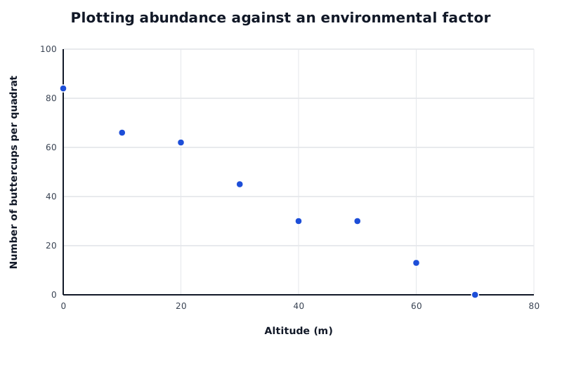
In this example, buttercup abundance generally decreases as altitude increases.
Data for Plotting abundance against an environmental factor
| Series | Altitude (m) | Number of buttercups per quadrat |
|---|---|---|
| Buttercup count | 0 | 84 |
| Buttercup count | 10 | 66 |
| Buttercup count | 20 | 62 |
| Buttercup count | 30 | 45 |
| Buttercup count | 40 | 30 |
| Buttercup count | 50 | 30 |
| Buttercup count | 60 | 13 |
| Buttercup count | 70 | 0 |
This dataset has altitudes from 0 to 70 m and buttercup counts from 0 to 84 per quadrat. Suitable scales would run from 0 to 70 m in 10 m intervals horizontally and from 0 to 90 buttercups in intervals of 10 vertically. The point means that the quadrat at an altitude of 30 m contained 45 buttercups.
The points show a general decrease in abundance as altitude increases. If asked for a line of best fit, draw a line or curve following the overall trend rather than joining every point. Do not automatically join the points on a scatter graph. Describe the overall relationship while recognising variation in the individual results.
A small number of quadrats may miss dense patches or bare areas. More randomly located samples generally give a more representative population estimate. Consistent species identification, quadrat area and counting rules make results comparable.
A transect examines only one strip of a habitat, so repeating it in different positions strengthens the evidence. Measuring the environmental factor at each quadrat is more informative than assuming it changes steadily with distance. Other changing factors remain a limitation when explaining the relationship.
Carry out fieldwork with minimal disturbance: avoid trampling the sampling area unnecessarily and do not uproot plants to count them.
Get unlimited access to all revision notes, key terms, and exam tips.
Describe random placement using random coordinates, not by throwing a quadrat or choosing places that look representative.
Count individuals of the named species, not the number of different species present.
Include quadrats containing zero individuals when calculating the mean.
Convert quadrat dimensions to metres before calculating an area in m². A 25 cm × 25 cm quadrat has an area of 0.0625 m².
For graphs, use labelled axes with units where appropriate and evenly spaced numerical scales. Draw the line requested: a line of best fit is not a dot-to-dot line.
Explain improvements specifically: more randomly located quadrats make the sample more representative; repeated transects test whether a pattern occurs elsewhere.
Population
All the organisms of one species living in a particular habitat.
Abundance
The number of individuals of a species in an area, sometimes expressed per unit area.
Distribution
The pattern of where a species occurs within an area.
Quadrat
A frame enclosing a known area, used to sample organisms such as plants or slow-moving animals.
Random sampling
Choosing sample locations by chance rather than personal preference, to reduce selection bias.
Transect
A line across a habitat along which organisms are recorded, directly or using quadrats, to investigate changes in distribution.
Abiotic factor
A non-living environmental condition, such as light intensity, temperature or soil moisture.
Arithmetic mean
The sum of all values divided by the number of values.
Median
The middle value after the data have been put in order; for an even number of values, the mean of the two middle values.
Mode
The value that occurs most often in a dataset.
Put your knowledge into practice — try past paper questions for Combined Science Trilogy
Population
All the organisms of one species living in a particular habitat.
Abundance
The number of individuals of a species in an area, sometimes expressed per unit area.
Distribution
The pattern of where a species occurs within an area.
Quadrat
A frame enclosing a known area, used to sample organisms such as plants or slow-moving animals.
Random sampling
Choosing sample locations by chance rather than personal preference, to reduce selection bias.
Transect
A line across a habitat along which organisms are recorded, directly or using quadrats, to investigate changes in distribution.
Abiotic factor
A non-living environmental condition, such as light intensity, temperature or soil moisture.
Arithmetic mean
The sum of all values divided by the number of values.
Median
The middle value after the data have been put in order; for an even number of values, the mean of the two middle values.
Mode
The value that occurs most often in a dataset.
Use matching area units. Median: order the values and find the middle; average the two middle values for an even-sized dataset. Mode: most frequent value.
Get unlimited access to all revision notes, key terms, and exam tips.