

Loading…
Loading…
Loading…
OCR GCSE Psychology · J203
OCR J203 · Handling Data Check the specification (PDF) (opens in a new tab)
Psychologists collect scores, counts and measurements to investigate behaviour. A table preserves numerical detail, while a graph can make comparisons and patterns easier to see. The choice of display depends on what the numbers represent.
Separate categories, such as reading and talking, suit a bar chart. Measurements on a continuous scale, such as reaction time, can be grouped into intervals and shown in a histogram. A pie chart shows how categories contribute to a total. A line graph shows change across a continuous scale, while a scatter diagram shows the relationship between two measured variables.
Before drawing a graph, decide what belongs on each axis. Give it an informative title, label the axes with the measurements and their units, and choose evenly spaced numerical scales that accommodate the data. These labels tell the reader what the pattern actually means.
A frequency is the number of times a value or category occurs. A frequency table summarises these counts rather than listing every observation separately.
During a structured observation, a researcher can use a tally chart with columns headed category of behaviour, tally and total. Each time a behaviour occurs, one tally mark is added to its row. Tally marks are grouped in fives: four upright strokes, with a fifth stroke drawn across them. This makes the final count quicker to check.
An observation of university students' study behaviours can be summarised as follows:
| Category of behaviour | Total frequency |
|---|---|
| Reading | 6 |
| Talking | 4 |
| Writing | 11 |
| Using phone | 2 |
The reading row would contain a group of five tally marks and one extra mark; writing would contain two groups of five and one extra. The frequencies add to recorded instances of behaviour. This need not mean 23 different students: a person may contribute more than one observation.
To interpret the table, compare frequencies. Writing occurred most often, with 11 instances, and phone use least often, with two. Reading occurred two more times than talking. These are conclusions about what was recorded, not explanations of why students behaved that way.
A bar chart represents each category with a separate bar. Put the categories on the horizontal, or -axis, and frequency on the vertical, or -axis. For the study-behaviour table, draw bars reaching 6, 4, 11 and 2. Make them equal in width, with equal gaps between them: the gaps show that the categories are separate.
To convert the chart back into a table, find the top of each bar, follow it across to the vertical scale and record its value beside the category name. Drawing and reading are therefore opposite directions of the same process: table values determine bar heights, and bar heights allow the values to be recovered.
Bar charts can also compare mean scores, rather than counts. For example, a chart could compare mean reaction time for a group given caffeine and a group without caffeine. Its vertical axis would be labelled mean reaction time in seconds. A lower bar would mean a shorter average reaction time, not fewer participants.
Continuous data can take any value within a range. A reaction time, for example, might be 0.32 seconds or 0.327 seconds, depending on the precision of the measurement. A histogram groups such measurements into intervals.
Suppose 30 pupils complete a reaction-time task and their times are grouped as follows:
| Reaction time, (seconds) | Frequency |
|---|---|
| 4 | |
| 11 | |
The interval notation means that the lower boundary is included and the upper boundary is excluded. A time of exactly 0.3 seconds goes in the second interval, so it is not counted twice.
To draw the histogram, mark the interval boundaries on the horizontal time scale. Each interval is 0.1 seconds wide. Put frequency on the vertical axis and draw touching bars at heights 4, 11, 9 and 6. The bars touch because the measurement scale continues from one interval into the next.
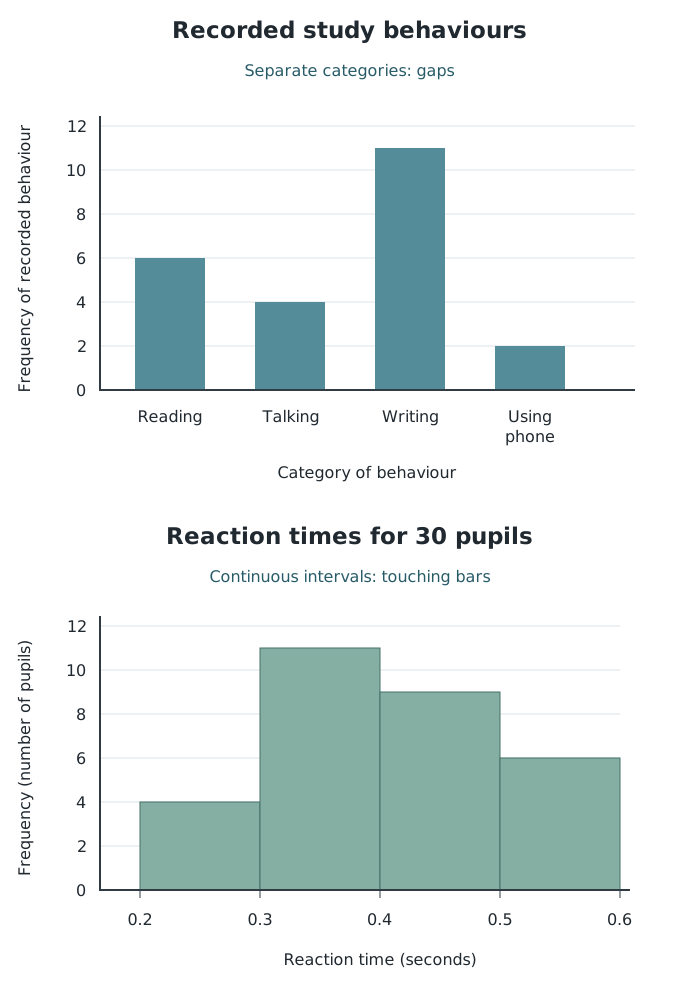
Separate categories have gaps between bars; continuous measurement intervals meet without gaps.
The tallest histogram bar shows that the most frequent reaction-time interval is from 0.3 up to, but not including, 0.4 seconds. Adding the first two frequencies shows that 15 pupils reacted in less than 0.4 seconds. All four frequencies total 30.
Grouping makes the overall pattern clearer but loses some detail. The histogram tells us that 11 times fell in the second interval; it does not reveal each pupil's exact time. The frequency-height method here uses equal-width intervals.
A pie chart divides a circle into sectors, with each sector representing a category's share of the total. It is most readable with a small number of categories, around six or fewer. Larger proportions produce larger sectors.
Because a full circle contains , calculate each sector using:
For the study-behaviour counts, reading accounts for six of the 23 observations. Its sector angle is . Calculate the other angles in the same way, then use a protractor to draw and label the sectors. The completed sectors should fill the circle.
To translate a sector back into a frequency, divide its angle by and multiply by the total. The total matters: half a circle represents half the observations, but that could mean 10 observations out of 20 or 100 out of 200.
A line graph plots values against a continuous scale, such as time, and joins the points in order. A rising section indicates an increase; a falling section indicates a decrease. Two lines can make it easier to compare conditions at the same time points.
Suppose a memory experiment produces these mean recall scores:
| Time after learning (hours) | Memory aid A: mean items recalled | Memory aid B: mean items recalled |
|---|---|---|
| 1 | 18 | 12 |
| 2 | 12 | 15 |
| 3 | 25 | 21 |
| 4 | 21 | 8 |
Put time in hours on the horizontal axis and mean number of items recalled on the vertical axis. Plot the four points for aid A and join them in time order, then do the same for aid B. Use distinct lines and a key identifying each aid.
At two hours, aid B has the higher mean recall score: 15 compared with 12. At four hours, aid A is higher by 13 items. Neither line rises steadily across all four measurements. Interpretation means describing the actual pattern, rather than assuming that scores must always increase or decrease.
A line graph can also represent grouped frequency data by plotting the frequency at the midpoint of each interval and joining those points.
A scatter diagram plots paired measurements of two variables. Each point represents one pair of scores, such as one pupil's daily screen time and their sleep duration. Put one variable on each axis and plot the point where its two values meet.
Suppose six pupils have the following pairs of measurements:
| Daily screen time (hours) | Sleep duration (hours) |
|---|---|
| 2 | 9.0 |
| 3 | 8.0 |
| 4 | 8.5 |
| 5 | 7.0 |
| 6 | 7.5 |
| 7 | 6.5 |
For the pupil with five hours of screen time and seven hours of sleep, move to 5 on the horizontal axis and 7 on the vertical axis, then mark their intersection. Repeat this for every pair, keeping the points separate.
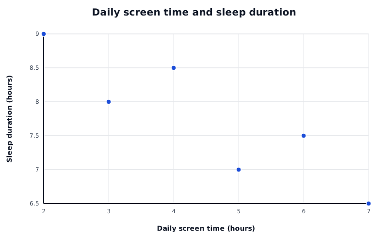
Each point represents one pupil's paired measurements. The overall downward pattern shows a negative correlation.
Data for Daily screen time and sleep duration
| Series | Daily screen time (hours) | Sleep duration (hours) |
|---|---|---|
| Pupils | 2 | 9 |
| Pupils | 3 | 8 |
| Pupils | 4 | 8.5 |
| Pupils | 5 | 7 |
| Pupils | 6 | 7.5 |
| Pupils | 7 | 6.5 |
Read the overall pattern from left to right:
In this example, higher screen time generally accompanies shorter sleep duration, so the correlation is negative. The points do not need to lie perfectly on a line for a relationship to exist. A tighter pattern around a rising or falling line indicates a stronger relationship than a widely scattered pattern.
A correlation describes an association, not necessarily a cause. This graph alone cannot establish that screen time reduces sleep: the direction of any influence is uncertain, and another factor could affect both variables.
A distribution describes how scores are spread across their possible values. A normal distribution has a symmetrical bell shape: most scores cluster around the centre, with fewer scores towards either extreme.
In an ideal normal distribution, the mean, median and mode are all at the same central point. Half the scores lie to the left of the centre and half lie to the right. The two sides mirror one another.
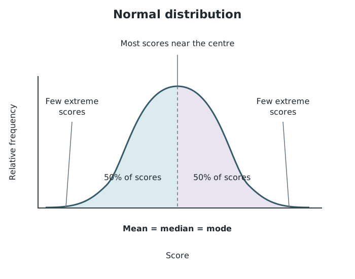
A normal distribution is symmetrical, with most scores near the centre and half on each side.
IQ scores provide a familiar example: they are commonly assumed to be normally distributed around a mean of 100. Scores close to 100 are more common than scores far above or below it.
When inspecting a distribution, look for the combination of a central peak, fewer extreme scores and symmetry. A peak on its own is not enough to establish a normal distribution, and not every psychological dataset follows this pattern.
| Display | Main use |
|---|---|
| Frequency table | Counts for values, categories or intervals |
| Bar chart | Separate categories; frequencies or means |
| Histogram | Continuous measurements grouped into intervals |
| Pie chart |
Give graphs an informative title, label both axes and include units where relevant. Use evenly spaced numerical scales.
Keep bar-chart bars equal in width with equal gaps. For a histogram with equal-width intervals, draw touching bars with frequency on the vertical axis.
Check that a frequency table's total matches the number of observations or scores, not necessarily the number of participants.
Plot each pair of scores as one point on a scatter diagram; do not join the points.
When interpreting a correlation, name its direction and explain it using the two variables. Do not claim that correlation proves causation.
Read the vertical-axis label before interpreting a bar: its height may represent a frequency or a mean.
It can see this note and what your specification asks for.
Answers are free with an account.
1 free note left this week
Get more free notesYour answer sets when this note comes back for review, or marks it complete.
Was this note helpful?
Log in to tell us whether it helped, or to report a problem.
Last updated
Frequency
The number of times a particular value or category occurs in a dataset.
Frequency table
A table showing how often each value, category or interval occurs in a dataset.
Tally chart
A table used to record occurrences as they happen, using tally marks that are counted to obtain frequencies.
Bar chart
A chart comparing separate categories using equal-width bars with gaps between them. Bar heights represent values such as frequencies or means.
Continuous data
Data measured on a scale that can take any value within a range, such as time in seconds.
Histogram
A graph displaying continuous data grouped into intervals, with touching bars. For equal-width intervals, bar heights show frequencies.
Pie chart
A circular chart divided into sectors showing each category's proportion of a total.
Line graph
A graph with points joined in order to show how a measurement changes across a continuous scale, such as time.
Scatter diagram
A graph plotting paired measurements of two variables, with one point for each pair, to reveal a possible relationship.
Correlation
A relationship between two variables in which their values tend to vary together. A correlation alone does not establish cause and effect.
Normal distribution
A symmetrical, bell-shaped distribution in which most scores cluster around the centre, where the mean, median and mode coincide.
Put your knowledge into practice — try past paper questions for Psychology
Frequency
The number of times a particular value or category occurs in a dataset.
Frequency table
A table showing how often each value, category or interval occurs in a dataset.
Tally chart
A table used to record occurrences as they happen, using tally marks that are counted to obtain frequencies.
Bar chart
A chart comparing separate categories using equal-width bars with gaps between them. Bar heights represent values such as frequencies or means.
Continuous data
Data measured on a scale that can take any value within a range, such as time in seconds.
Histogram
A graph displaying continuous data grouped into intervals, with touching bars. For equal-width intervals, bar heights show frequencies.
Pie chart
A circular chart divided into sectors showing each category's proportion of a total.
Line graph
A graph with points joined in order to show how a measurement changes across a continuous scale, such as time.
Scatter diagram
A graph plotting paired measurements of two variables, with one point for each pair, to reveal a possible relationship.
Correlation
A relationship between two variables in which their values tend to vary together. A correlation alone does not establish cause and effect.
Normal distribution
A symmetrical, bell-shaped distribution in which most scores cluster around the centre, where the mean, median and mode coincide.
| 9 |
| 6 |
| Categories' shares of a total |
| Line graph | Change across a continuous scale; comparison of conditions |
| Scatter diagram | Relationship between paired measurements |
Bar chart: equal-width bars with gaps. Histogram: touching bars; for equal-width intervals, height shows frequency.
Symmetrical bell shape; most scores near the centre; few at either extreme. Mean, median and mode coincide at the centre, with 50% of scores on each side.