

Loading…
Loading…
Loading…
OCR GCSE Combined Science B · J260
OCR J260 · M2 Handling Data Check the specification (PDF) (opens in a new tab)
A scientific investigation can produce many readings. A list preserves individual measurements, but a summary helps us compare results and spot patterns. An average describes a typical value; a frequency table shows how often values occur; a graph makes the pattern easier to see.
Quantitative data are numerical data, such as a plant’s height, a reaction time or the number of organisms counted. The kind of data and the question being investigated determine which summary is useful.
The arithmetic mean uses every value. Add all the readings, then divide by the number of readings:
Suppose five seedlings have heights of 2, 3, 3, 4 and 8 cm. Their total height is 20 cm, so their mean height is . The mean has the same unit as the original measurements. It need not be a value that occurs in the data.
The median is the middle value after the readings have been put in numerical order. These five heights are already ordered, so the third value, 3 cm, is the median: two readings lie on either side of it. With an even number of readings, there are two middle values. For example, the median of 2, 3, 5 and 8 cm is .
The mode is the most frequent value. In the five-seedling example, 3 cm occurs twice, while every other height occurs once, so the mode is 3 cm. A data set can have more than one mode if values tie for the highest frequency, or no mode if no value occurs more often than the others.
These averages answer slightly different questions. The mean takes account of every measurement, but an unusually large or small reading can pull it towards that value. The median depends on the position of the middle readings, so it is less affected by extreme values. The mode identifies the most common result. Here, the 8 cm seedling helps explain why the mean is higher than the median and mode.
Frequency means how often something occurs. To construct a frequency table, list the possible values or categories, count each observation once, and record the totals. Tally marks can help: group them in fives so that they are easy to count.
For the five seedling heights, the table is:
| Height / cm | Frequency |
|---|---|
| 2 | 1 |
| 3 | 2 |
| 4 | 1 |
| 8 | 1 |
| Total | 5 |
The frequency column tells us that two seedlings are 3 cm tall, not that their combined height is 2 cm. Adding the frequencies gives the total number of seedlings. The largest frequency identifies the modal height.
Continuous measurements, such as height or time, can take values between whole numbers. If there are many different readings, group them into class intervals rather than making a separate row for every measurement. Make the intervals non-overlapping so that a reading cannot belong to two groups.
For example, the same heights can be grouped as follows:
| Height, / cm | Frequency |
|---|---|
| 0 | |
| 3 | |
| 1 | |
| 0 | |
| 1 |
The interval includes 2 cm and 3 cm but excludes 4 cm. Grouping makes the distribution clearer, although the exact measurements within each interval are no longer visible.
A bar chart compares separate categories. For example, suppose a survey records 4 daisies, 7 dandelions and 3 buttercups. Put the species on the horizontal axis and the number counted on the vertical axis. Draw bars of equal width with equal gaps between them. Their heights show the frequencies. Dandelions are the most common category in this example.
A histogram shows continuous measurements grouped into numerical intervals. Put the measurement and its unit on the horizontal axis, and keep the intervals in numerical order. The bars touch because neighbouring intervals belong to one continuous scale. For equal-width intervals, as in the seedling table, bar height can show frequency directly.
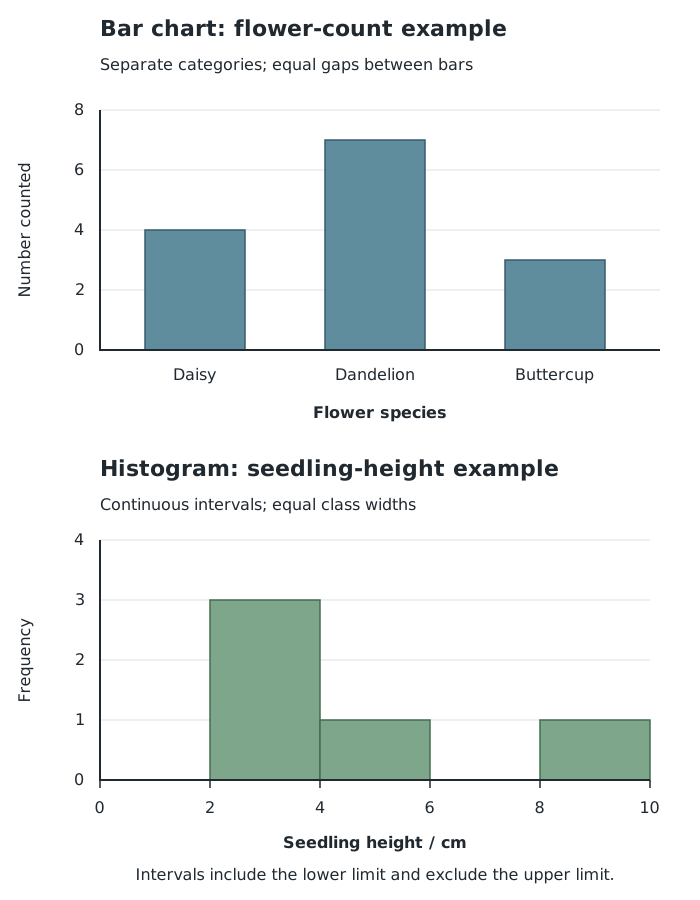
Separate bars compare categories; touching histogram bars show continuous measurements grouped into intervals.
To construct either graph, choose a useful title, label both axes and select a numerical scale that accommodates the data. Draw each bar to the correct height. For the seedling histogram, retain the empty intervals: leaving their positions visible shows where no measurements occurred.
When interpreting a graph, first read the axes and scale. Then identify the most common category or interval, compare frequencies and describe where measurements are concentrated. Here, three of the five seedlings are between 2 cm and just below 4 cm tall.
A scatter diagram displays paired measurements of two variables. Each point represents one pair, not a total or an average. Put one variable on the horizontal axis and the other on the vertical axis, label their units, and plot a cross where each pair of values meets. Do not join the points one after another.
Suppose temperature and gas volume are recorded for a fixed amount of gas at constant pressure. The following example shows how to plot and interpret such pairs.
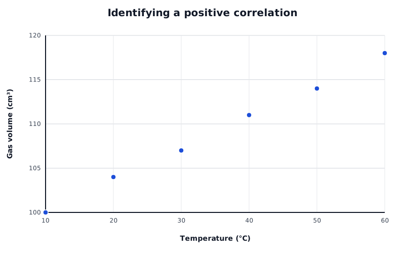
Example paired readings: gas volume tends to increase as temperature increases.
Data for Identifying a positive correlation
| Series | Temperature (°C) | Gas volume (cm³) |
|---|---|---|
| Example paired readings | 10 | 100 |
| Example paired readings | 20 | 104 |
| Example paired readings | 30 | 107 |
| Example paired readings | 40 | 111 |
| Example paired readings | 50 | 114 |
| Example paired readings | 60 | 118 |
A point at represents a temperature of 20 °C paired with a gas volume of 104 cm³. Across the graph, higher temperatures tend to occur with higher volumes: this is a positive correlation.
A negative correlation has the opposite pattern: as one variable increases, the other tends to decrease. With no correlation, the points show no clear overall relationship. For a roughly straight-line relationship, points clustered closely around an upward or downward trend indicate a stronger correlation than widely scattered points.
Describe the overall pattern rather than relying on one pair of points. A correlation is evidence of an association, but it does not by itself establish that changing one variable causes the other to change. The investigation’s conditions and other possible influences must also be considered.
Each point represents one paired measurement.
For a mean, divide by the number of readings, not by the number of different values.
Put values in order before finding the median. With an even number of values, average the two middle values.
Label graph axes with the quantity and its unit, where applicable, and use evenly spaced numerical scales.
Use separated bars for categories and touching bars for continuous class intervals.
Describe a correlation using both variables: for example, ‘As temperature increases, volume tends to increase.’ A correlation alone does not prove cause and effect.
It can see this note and what your specification asks for.
Answers are free with an account.
1 free note left this week
Get more free notesYour answer sets when this note comes back for review, or marks it complete.
Was this note helpful?
Log in to tell us whether it helped, or to report a problem.
Last updated
Arithmetic mean
The sum of all the values in a data set divided by the number of values.
Median
The middle value when data are arranged in numerical order; for an even number of values, it is the mean of the two middle values.
Mode
The value that occurs most frequently in a data set.
Frequency
The number of times a value or category occurs in a data set.
Frequency table
A table showing how often each value, category or class interval occurs.
Class interval
A numerical range used to group measurements, with boundaries that determine which values belong in it.
Bar chart
A graph with separate bars used to compare categories or distinct values.
Histogram
A graph showing the distribution of continuous numerical data grouped into intervals, with adjacent bars touching.
Scatter diagram
A graph in which each point represents a pair of values for two variables.
Correlation
An association between two variables, in which their values show a pattern of changing together.
Put your knowledge into practice — try past paper questions for Combined Science B
Arithmetic mean
The sum of all the values in a data set divided by the number of values.
Median
The middle value when data are arranged in numerical order; for an even number of values, it is the mean of the two middle values.
Mode
The value that occurs most frequently in a data set.
Frequency
The number of times a value or category occurs in a data set.
Frequency table
A table showing how often each value, category or class interval occurs.
Class interval
A numerical range used to group measurements, with boundaries that determine which values belong in it.
Bar chart
A graph with separate bars used to compare categories or distinct values.
Histogram
A graph showing the distribution of continuous numerical data grouped into intervals, with adjacent bars touching.
Scatter diagram
A graph in which each point represents a pair of values for two variables.
Correlation
An association between two variables, in which their values show a pattern of changing together.