

Loading…
Loading…
Loading…
AQA GCSE Statistics · 8382
AQA 8382 · 3.4.4 Check the specification (PDF) (opens in a new tab)
An average describes a typical value, but it does not tell us how much the values vary. A measure of spread, also called a measure of dispersion, describes how widely scattered the data values are.
When comparing datasets measuring the same quantity in the same units, a smaller spread indicates greater consistency. Different measures focus on different features: the range uses the two endpoints, the interquartile range uses the middle half, and standard deviation uses every value.
The range is the largest value minus the smallest value:
For a set of seed-germination times, the shortest time was 5 days and the longest was 23 days. The range was therefore days. This is a difference, not the interval ‘5 to 23 days’.
Range is quick to calculate, but it depends entirely on the two extreme values. It does not reveal how the remaining observations are distributed between them.
Quartiles divide ordered data into four approximately equal parts. The lower quartile, , marks about 25% of the data; the median, , marks about 50%; and the , , marks about 75%. These percentages describe dividing positions, so repeated values can prevent an exact percentage from lying strictly below a quartile.
First put the data in numerical order, retaining every repeated value. One way to find the quartiles is to locate the median, leave it out of both halves when the number of values is odd, and then find the median of each half. The median of the lower half is ; the median of the upper half is .
For the quartile calculations specified here, the number of observations, , is one less than a multiple of four, such as 7, 11 or 15. The quartile positions are therefore whole numbers:
For 11 observations, these positions are , and . Read the third, sixth and ninth values in the ordered list. The answers are the data values at those positions, not the numbers 3, 6 and 9 themselves.
The two methods agree here: excluding the sixth value leaves five values in each half. Their middle values are the third and ninth values of the original list. There is no need to interpolate between observations for these specified dataset sizes.
The interquartile range, or IQR, is the difference between the upper and :
In the seed-germination data, the lower quartile was 7 days and the upper quartile was 9 days. The IQR was days: the middle half of the germination times occupied a much narrower interval than the full dataset.
The 23-day germination time made the range large, while all the other times were between 5 and 11 days. The IQR better represents the spread of the central observations because it does not depend directly on the largest and smallest values. Moving an extreme endpoint further away, without changing the quartiles, changes the range but not the IQR.
Percentiles divide ordered data into 100 approximately equal parts. The 65th percentile marks the value at or below which approximately 65% of the observations lie. Percentiles are data values, not percentages themselves.
Quartiles are particular percentiles:
For grouped data, percentiles can be estimated from a cumulative frequency graph. Cumulative frequency is a running total: it counts observations up to each boundary. To find for observations, calculate the target cumulative frequency . Find that number on the vertical axis, move horizontally to the graph, then vertically down to the data-value axis.
The following quiz-time data show how this works:
| Time, (minutes) | Frequency | Cumulative frequency |
|---|---|---|
| 6 | 6 | |
| 24 | 30 |
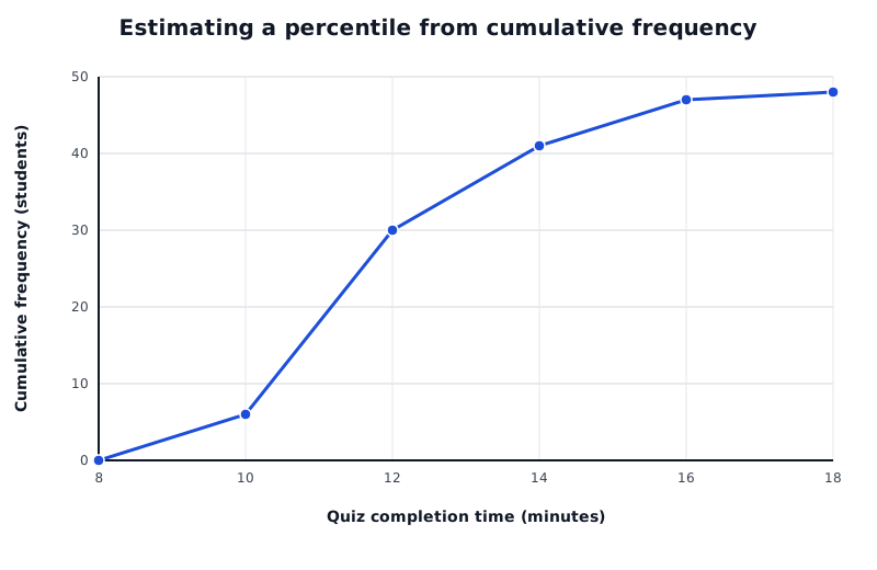
Cumulative frequencies from the grouped quiz times. The connecting lines allow percentile estimates; individual times within each class are unknown.
Data for Estimating a percentile from cumulative frequency
| Series | Quiz completion time (minutes) | Cumulative frequency (students) |
|---|---|---|
| Quiz completion times | 8 | 0 |
| Quiz completion times | 10 | 6 |
| Quiz completion times | 12 | 30 |
| Quiz completion times | 14 | 41 |
| Quiz completion times | 16 | 47 |
| Quiz completion times | 18 | 48 |
There are 48 students, so the target cumulative frequency for the 65th percentile is . The cumulative frequency rises from 30 to 41 in the interval , so the percentile lies in that interval. Reading the connecting line gives an estimate of about 12.2 minutes.
This is an estimate because the individual times within each interval are unknown. A straight line between class boundaries treats the observations as evenly distributed within that class. The same reading method transfers to other cumulative frequency graphs: calculate the target frequency first, then read the corresponding data value.
An interpercentile range is the difference between two specified percentiles. For example, the 30th-to-80th interpercentile range is . It measures the width of the interval containing approximately 50% of the observations between those dividing values. The 25th-to-75th interpercentile range is the IQR.
For pepper-harvest masses, the 2.5th percentile was 274.1 g and the 97.5th percentile was 532.4 g. The 2.5th-to-97.5th interpercentile range was g, describing the spread of the central 95% of the data.
Deciles divide ordered data into ten approximately equal parts. The first decile, , is , the second is , and so on. An is the difference between two specified deciles.
For the same harvest data, g and g. The first-to-ninth interdecile range was therefore g. This describes the spread of the central 80%. Other decile pairs can be used, so identify the pair before subtracting.
Standard deviation, usually written , measures spread around the mean using every observation. A small standard deviation indicates that values are generally close to the mean; a larger one indicates greater spread. Extreme values can affect it because every value enters the calculation.
A deviation is the difference between an observation and the mean. Simply adding these deviations would give zero: positive and negative deviations cancel. Squaring them prevents that cancellation. Standard deviation takes the square root of the average squared deviation:
Here, represents an observation, is the mean, is the number of observations, and means ‘add all of these terms’.
For the values 6, 9, 2, 11 and 5, the mean is :
| 6 | −0.6 | 0.36 |
| 9 | 2.4 | 5.76 |
The squared deviations total 49.2, so .
An equivalent formula is often quicker, especially when totals are supplied:
For the same values, and . Substitution gives , the same result.
Frequency tells us how many times a value occurs. Rather than writing out all the observations, multiply each contribution by its frequency, . The number of observations is , not the number of rows:
For a survey of rabbit owners, the calculation can be organised as follows:
| Number of rabbits, | Frequency, | ||
|---|---|---|---|
| 1 | 2 | 2 | 2 |
| 2 | 6 | 12 |
The mean is rabbits, and the standard deviation is rabbits. This describes spread around the mean; it is not the average number of rabbits owned.
Range, quartiles, percentile values, IQR, , and standard deviation all retain the units of the original data. For standard deviation, the final square root restores those units after the deviations have been squared.
For frequency data:
Smaller standard deviation means greater consistency around the mean. It uses every value and is sensitive to extremes. All spread measures above use the original data units.
Put raw data in numerical order before finding quartiles. A quartile position is not the quartile value: read the value at that position.
For the specified quartile datasets, n is one less than a multiple of 4. Use n + 1 when calculating quartile positions; no fractional-position adjustment is needed.
On a cumulative frequency graph, calculate the required percentage of the total frequency, not a percentage of the horizontal-axis values.
State which percentiles or deciles an interpercentile or interdecile range uses, and subtract the lower value from the higher value.
For standard deviation, distinguish the sum of squares from the square of the sum. Keep full calculator precision until the final answer.
Use the standard deviation calculation that divides by n, or by the total frequency, rather than the alternative calculation that divides by n − 1.
It can see this note and what your specification asks for.
Answers are free with an account.
1 free note left this week
Get more free notesYour answer sets when this note comes back for review, or marks it complete.
Was this note helpful?
Log in to tell us whether it helped, or to report a problem.
Last updated
Measure of spread
A numerical measure of how widely the values in a dataset are dispersed.
Range
The largest value minus the smallest value in a dataset.
Quartile
One of the three dividing values that split ordered data into four approximately equal parts.
Lower quartile
The value approximately one-quarter of the way through ordered data, also called the first quartile, , or the 25th percentile.
Upper quartile
The value approximately three-quarters of the way through ordered data, also called the third quartile, , or the 75th percentile.
Interquartile range
The upper quartile minus the lower quartile: . It measures the spread of the middle 50% of the data.
Percentile
A dividing value in ordered data. The th percentile, , marks approximately of the data at or below that value.
Decile
One of the nine dividing values that split ordered data into ten approximately equal parts. The th decile is the th percentile.
Interpercentile range
The difference between two specified percentiles of a dataset.
Interdecile range
The difference between two specified deciles of a dataset.
Standard deviation
A measure of spread around the mean, calculated by taking the square root of the mean squared deviation from the mean.
Put your knowledge into practice — try past paper questions for Statistics
Measure of spread
A numerical measure of how widely the values in a dataset are dispersed.
Range
The largest value minus the smallest value in a dataset.
Quartile
One of the three dividing values that split ordered data into four approximately equal parts.
Lower quartile
The value approximately one-quarter of the way through ordered data, also called the first quartile, , or the 25th percentile.
Upper quartile
The value approximately three-quarters of the way through ordered data, also called the third quartile, , or the 75th percentile.
Interquartile range
The upper quartile minus the lower quartile: . It measures the spread of the middle 50% of the data.
Percentile
A dividing value in ordered data. The th percentile, , marks approximately of the data at or below that value.
Decile
One of the nine dividing values that split ordered data into ten approximately equal parts. The th decile is the th percentile.
Interpercentile range
The difference between two specified percentiles of a dataset.
Interdecile range
The difference between two specified deciles of a dataset.
Standard deviation
A measure of spread around the mean, calculated by taking the square root of the mean squared deviation from the mean.
| 11 | 41 |
| 6 | 47 |
| 1 | 48 |
| 2 | −4.6 | 21.16 |
| 11 | 4.4 | 19.36 |
| 5 | −1.6 | 2.56 |
| 24 |
| 3 | 4 | 12 | 36 |
| 4 | 6 | 24 | 96 |
| 5 | 2 | 10 | 50 |
| Total | 20 | 60 | 208 |